HETGS Line Profiles

Building the LSF library for Chandra CALDB

Assumptions for building LSF

There are three major assumptions that we make to build the LSF library for Chandra CALDB:

MARX provides a perfect description of Chandra grating instruments,
CIAO/DS tools perform tasks as designed,
the HRMA system (e.g., focus) is stable in a long run.

If any of these criteria is not met, the LSF library products may not be valid or suitable for science analysis. For example, when minor changes in the MARX internal HRMA system are required based on new Chandra calibrations, we will need to refine our tools and rebuild the LSF library.

Steps for Building LSF

The steps to build LSFs are as follows:

Run MARX simulations for mono-energetic beams,
Generate a 2-D histogram of photon distribution per grating per order from MARX simulated dataset,
Per a fixed extraction width, generate an integrated 1-D line profile from the 2-D histogram image,
Perform multi-component fitting (2 Gaussian + 2 Lorentzian) to parameterize the 1-D profile,
Evaluate encircled energy fraction,
Repeat this process for various energy values and extraction widths,
Record and tabulate the measured values; interpolate them with uniform grid points later,
Bundle the interpolated values into a FITS file.

Examples of Line Profile fitting

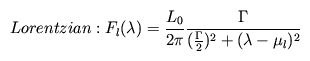
Earlier on 1-D line profiles were fitted with one Gaussian and one Lorentzian functions for ACIS-S/HETG. However we note that these 2-component fit do not provide adequate description of the profile in general. Hence two Gaussian and two Lorentzian functions are now being utilized.

Gaussian and Lorentzian functions are defined an in the following forms:

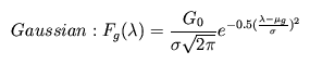
$Gaussian: F_g(\lambda) = {{G_0}\over{{\sigma}\sqrt{2\pi}}} e^{-0.5({{\lambda-{{\mu}_g}}\over{\sigma}})^2}$ $Lorentzian: F_l(\lambda) = {{L_0}\over{2\pi}}{{{\Gamma}\over{({\Gamma\over{2}})^2 + (\lambda - {{\mu}_l})^2}}}$ where G_0

and

refers to Gaussian and Lorentzian amplitude terms, ${\mu}_g$ and ${\mu}_l$ represent line centroid positions for Gaussian and Lorentzian component respectively, $\sigma$ and $\Gamma$ are Gaussian and Lorentzian widths. These are expressed as a function of wavelength, $\lambda$ .

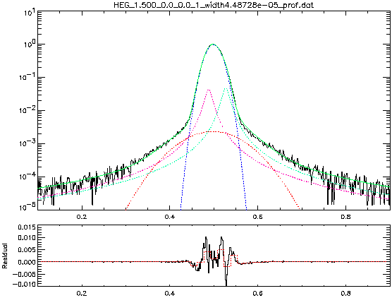
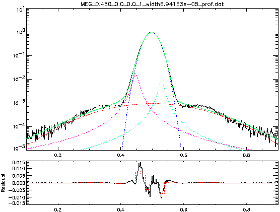
Figure 2 illustrate the fitting process with the four-component fitting:

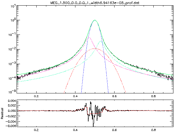
Figure 2: HEG (top) and MEG (bottom) +1 order LSF at E = 1.5keV. Each line profile is fitted with 2 Gaussian (color-coded as blue and red lines) and 2 Lorentzian (emerald green and purple) functions. Gaussian 1 component, shown in blue, dictates the goodness of the fit at its core of LSF. The sum of these functions (light-green) is compared with the real line profile and then the residual (its scale being given in percentage in the bottom of the panel) is derived to show the fidelty of the fitting process.

Generally the four-component fitting suffices to describe both its core and wing part of LSFs. However sometimes even the four-component fitting is not sufficient, especially for the MEG line profile at a lower E value. Figure 3 gives this worst example:

Figure 3: MEG +1 order LSF at E = 450eV. This example shows that even four-component fitting sometimes does not give a decent description of instrumental line profile.

The users should be aware that the LSF library may include such imperfection.

This fitting process was repeated roughly at 20+ different energies per extraction width. Figure 4 shows primary Gaussian widths as a function of energy at the extraction width ~ 9.2'' (~+/- 0.00129 degrees):

Derived line widths for Gaussian <strong>1</strong> Component of HEG

Derived line widths for Gaussian <strong>1</strong> Component of MEG

Figure 4: Measured line widths for Gaussian 1 Component per a fixed extraction width at various energies. (Top): HEG; (Bottom): MEG. This measurement is repeated five times for different extraction widths.

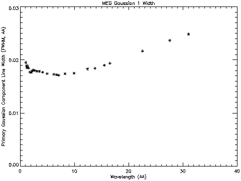
The fitting parameters for amplitude, line position, and width for both two Gaussian and two Lorentzian functions -- i.e., a total of 12 parameters -- are measured and recorded to build the LSF library.

Encircled Energy Fraction (EEFRACS)

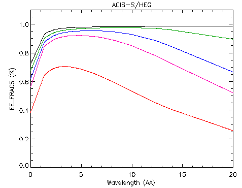
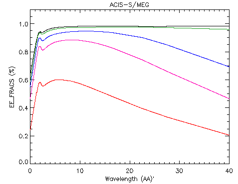
We define the term "encircled energy fraction" (EEFRACS) as the ratio of the sum of counts included in the extraction region to the total counts detected on the detector per mono-energetic beam per order. We can evaluate this numerically in MARX simulations. Figure 5 shows the EEFRACS as a function of wavelength for both HEG and MEG:

$Encircled energy fraction vs. wavelength for HEG.$

$Encircled energy fraction vs. wavelength for MEG.$ Figure 5: Encircled energy fraction vs. Wavelength per extraction width. (Top): HEG (black ~ +/-0.0013, green ~ +/-0.00051, blue ~ +/- 0.00035, purple ~ +/-0.00028, and red ~ +/-0.00015 degrees for extraction widths); (bottom): MEG (black ~ +/-0.002, green ~ +/-0.00094, blue ~ +/- 0.00042, purple ~ +/-0.00027, and red ~ +/-0.00012 degrees for extraction widths).

Final Step

All the fitting parameters plus EEFRACS values are tabulated first, and then interpolated with uniform grid points. Then the array of data values are written into a FITS file that meets the requirement of Chandra CALDB. This concludes the building process of the LSF library. [Note that all the tools for making the LSF library can be made available to the public, if they wish to duplicate the effort. However, technical support for such is not provided (but moral support may be).]

The next section describes caveats associated with the use of the LSF library.

Previous: Generation of LSF Reference Data Next: Caveats on Using LSF

This page was last updated Dec 4, 2002 by Bish K. Ishibashi. To comment on it or the material presented here, send email to bish (at) space.mit.edu.