Although Compute an HRC-I Exposure Map and Build Fluxed Image explains how to a HRC-I fluxed map in detail, we explain in this note how to incorporate a stowed background map to create a better fluxed map. The "ring" artifacts mentioned in the flux map are due to applying a HRMA vignetting correction to the particle background. Subtracting an estimate for the particle background from the observation before exposure correcting should eliminate these artifacts. If you like to know more about HRC stowed backgrounds, please go to High Resolution Camera Stowed Background Study.
The following table shows the yearly cumulative HRC-I stowed level 1 event file links and their dead time corrected total yearly exposure time.
| Year | HRC I Evt1 File | Corrected Exposure Time (sec) | Total Event Numbers |
|---|---|---|---|
| 2000 | hrc_i_115_2000 evt1 file | 94,292 | 3,907,097 |
| 2001 | hrc_i_115_2001 evt1 file | 67,258 | 3,070,201 |
| 2002 | hrc_i_115_2002 evt1 file | 70,560 | 3,312,125 |
| 2003 | hrc_i_115_2003 evt1 file | 38,267 | 1,838,713 |
| 2004 | hrc_i_115_2004 evt1 file | 42,471 | 2,717,713 |
| 2005 | hrc_i_115_2005 evt1 file | 42,450 | 2,768,383 |
| 2006 | hrc_i_115_2006 evt1 file | 33,920 | 2,724,371 |
| 2007 | hrc_i_115_2007 evt1 file | 47,738 | 4,539,941 |
| 2008 | hrc_i_115_2008 evt1 file | 37,129 | 3,976,703 |
| 2009 | hrc_i_115_2009 evt1 file | 32,445 | 4,078,590 |
| 2010 | hrc_i_115_2010 evt1 file | 16,468 | 1,967,995 |
| 2011 | hrc_i_115_2011 evt1 file | 32,467 | 3,537,743 |
| 2012 | hrc_i_115_2012 evt1 file | 19,807 | 1,934,917 |
| 2013 | hrc_i_115_2013 evt1 file | 51,682 | 4,682,604 |
| 2014 | hrc_i_115_2014 evt1 file | 28,793 | 2,427,420 |
| 2015 | hrc_i_115_2015 evt1 file | 14,356 | 1,337,910 |
| 2016 | hrc_i_115_2016 evt1 file | 16,942 | 2,661,755 |
| 2017 | hrc_i_115_2017 evt1 file | 19,774 | 3,111,414 |
| 2018 | hrc_i_115_2018 evt1 file | 9,200 | 1,497,558 |
| 2019 | hrc_i_115_2019 evt1 file | 14,611 | 2,457,233 |
| 2020 | hrc_i_115_2020 evt1 file | 13,630 | 1,977,865 |
| 2021 | hrc_i_115_2021 evt1 file | 32,571 | 4,672,490 |
| 2022 | hrc_i_115_2022 evt1 file | 2,161 | 0 |
The HRC-I background event files are also available for download as part of CALDB 4.7.3, released on 31 May 2016. (see also CIAO The HRC-I Background Event Files Page.)
Download the event file of the year in which your observation is done. If the observation is done during the current year, you may want to combine the current year and the previous year to have a sufficient stowed observation time. Since the thread Compute an HRC-I Exposure Map and Build Fluxed Image uses OBSID = 144, observed in year 2000, we use the year 2000 stowed background data in the example below.
First, we perform status-bit filtering on the stowed background data.This filtering will remove the events that standard processing would have removeded as likely "background" events in generating the primary (level 2) event list.
unix% dmcopy "hrc_i_115_2000_evt1.fits[status=xxxxxx00xxxx0xxx00000000x0000000]" \
      outfile=hrc_i_115_2000_evt2.fits
If a different status-bit mask was used, the corresponding change should be made here as well.
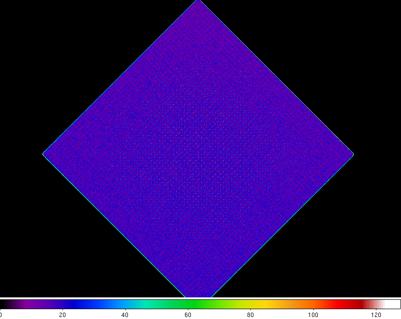
Figure 1: Stowed Background Image before (Left) and after Status Bit Correction
Since the stowed event file does not have correct sky coordinates, we need to add them; we will do this using the CIAO tool "reproject_events". For HRC event-lists a time column is required and the times need to lie within the observation's time-interval. We use the CIAO tool dmtcalc to modify the background file's event-times to match those in the GTI of the observation.
Using the observation's event list, hrcf00144N004_evt2.fits, to get the times:
unix% dmstat "hrcf00144N004_evt2.fits[cols time]"
time[s]
    min:        84154932.677          @:        1
    max:        84185127.061          @:        854440
   mean:        84169382.053
  sigma:        9148.9938848
    sum:        7.1917686801e+13
   good:        854440
   null:        0
we can then use dmtcalc modify the stowed background event times:
unix% dmtcalc infile=hrc_i_115_2000_evt2.fits outfile=hrc_i_115_2000_time_corrected_evt2.fits \
      expression="time=30194*#trand+84154933"
where
Now, using reproject_events and the aspect file of obsid 144, we compute the sky coordinates matched to chip coordinates of the stowed background file.
unix% reproject_events infile="hrc_i_115_2000_time_corrected_evt2.fits" \
      outfile=hrc_i_115_2000_bkg.fits aspect=pcadf084154631N004_asol1.fits \
      match=hrcf00144N004_evt2.fits random=0 clobber=yes
Since "HRC-I Exposure Map and Fluxed Image" is using the binning of 32x32, we use the same factor.
unix% dmcopy "hrc_i_115_2000_bkg.fits[bin x=::32, y=::32]" outfile=hrc_i_115_2000_bkg_img.fits
Subtract this background image from the observation image, using a suitable weight to account for the difference in exposure times.
unix% dmimgcalc 144_img32.fits hrc_i_115_2000_bkg_img.fits 144_img32_bkg_sub.fits \
      sub weight=1 weight2=0.3202
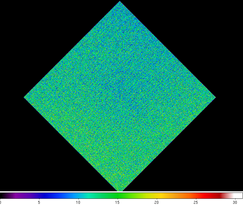
where 0.3202 is (observation exposure time)/(background exposure time)= 30192/94287. The background subtracted image is shown below. From this image, all negative value pixels were droped.
Figure 2: The Background Subtracted Observation Image
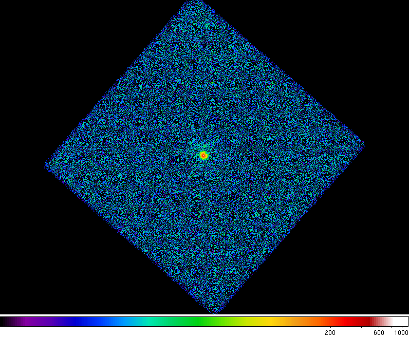
On this image, we apply the exposure map normalization, following the example shown in HRC-I Exposure Map and Fluxed Image page.
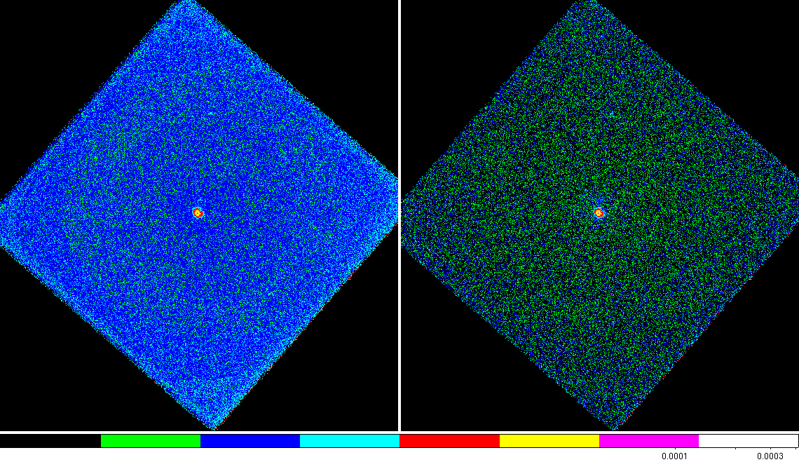
The resulting fluxed image is shown below (the right side plot). As before, all negative value pixels were droped from the map.
Figure 3: Fluxed Image without (Left) and with the Background Correction
The images below are same as above, but the upper threshold is set to 3.0e-5 (cnt/pix/sec) to show the concentric rings on the original data analysis (left). The background subrtracted image (right) does not show these rings.
Figure 4: Fluxed Image without (Left) and with the Background Correction with upper threshold set to 3.0e-5 (cnt/pix/sec)
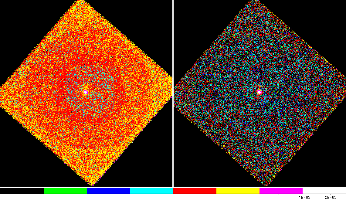
Figure 5: Fluxed Image of the Central Part without (Left) and with the Background Correction
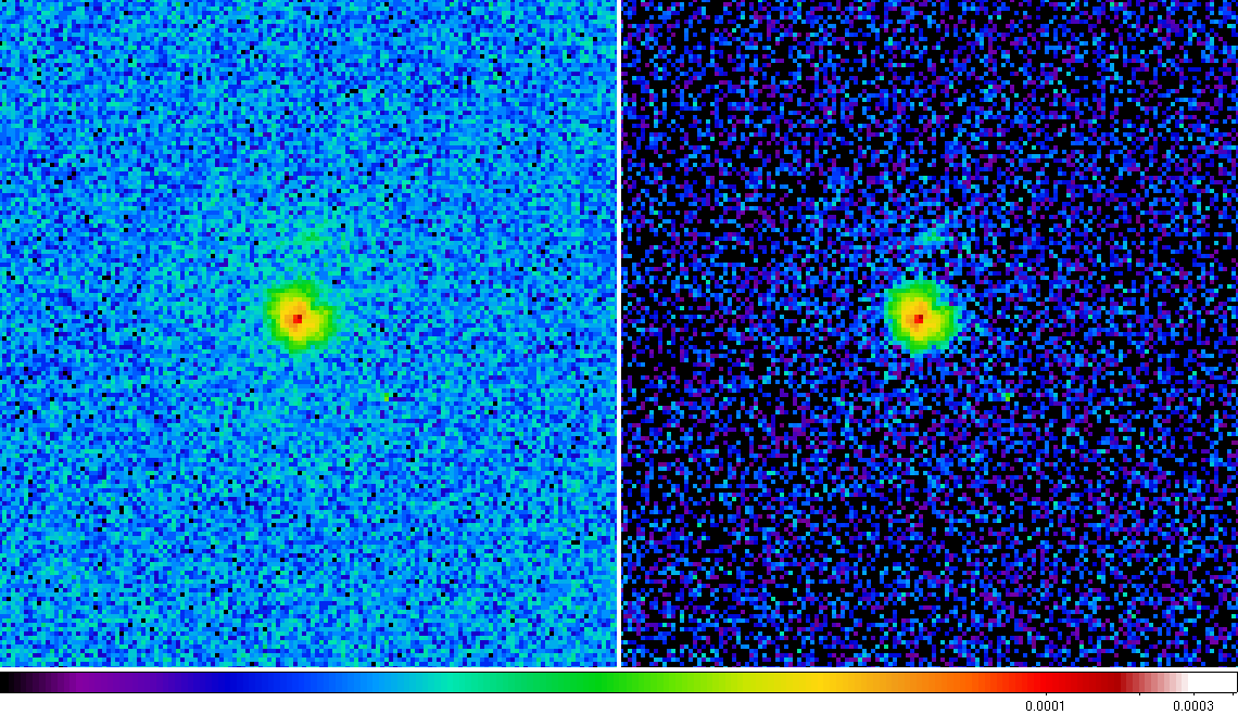
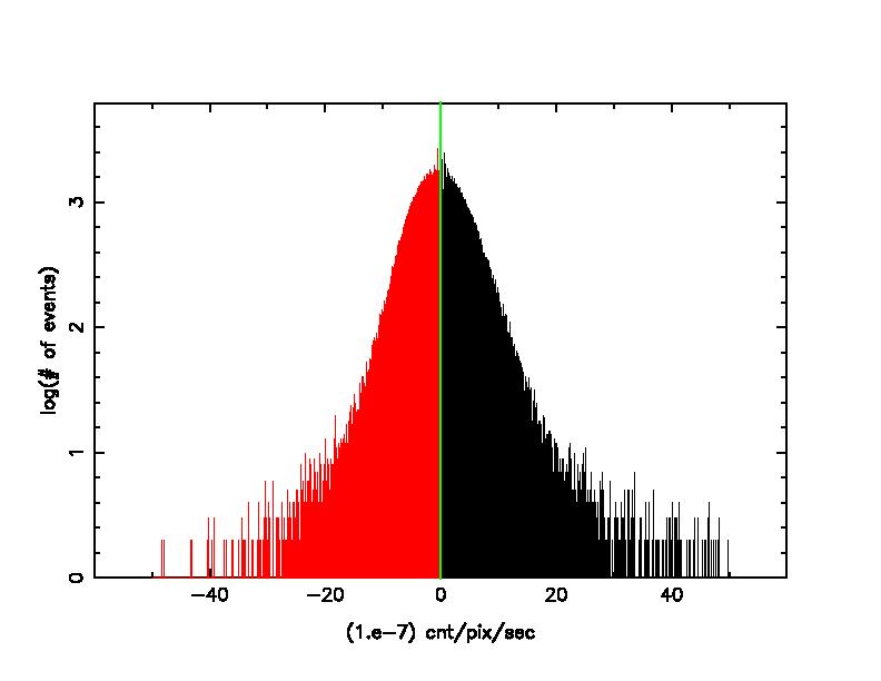
Figure 6 is the plot of the numbers of events for counts/pixel/sec after the background adjusted. About a half of the events are in the negative side. This is statistically expected.
The background file binned at 32x32 probably has a significant number of counts in each image cell (mean ~2e-7cnt/pix/sec). The observation when binned at the same factor may have many image cells with zero events, some with one and a few with two or more. The cells with zero will give negative values in the difference map but the cells with ones or more give positive values and on average, away from sources we can expect the difference to be zero or slightly larger due to an additional sky- or low-energy-proton- background component in the observation.
Figure 6: # of Events for Counts/Pixel/Sec after Background Adjusted