Next: 5. Sherpa Models Up: Sherpa Reference Manual Previous: 3. Sherpa Filtering
The primary task of Sherpa is to fit a model
![]() to a set of observed data, where
to a set of observed data, where
![]() denotes the model parameters. An
optimization method is one that is used to
determine the vector of model parameter
values,
denotes the model parameters. An
optimization method is one that is used to
determine the vector of model parameter
values,
![]() , for which
the chosen fit statistic is minimized.
, for which
the chosen fit statistic is minimized.
Optimization is complicated because there is no guarantee that, for a given model and dataset, there will not be multiple local fit-statistic minima. Thus Sherpa provides a number of optimization methods, each of which has different advantages and disadvantages. The default optimization method is POWELL, which is a robust method for finding the nearest local fit-statistic minimum (but not necessarily the global minimum). The user can change the method using the METHOD | SEARCHMETHOD command. For example, to change the optimization method to SIMPLEX:
sherpa> METHOD SIMPLEX
Below, we provide a fuller discussion of the relative merits of
different optimization methods, and then describe each of Sherpa
optimization methods in turn.
Each method section includes a description
of the method, and a table listing of the method parameters.
The listing of method parameters includes the Sherpa parameter number,
and the corresponding Sherpa parameter name (![]() paramname
paramname![]() ).
).
The contents of this section are taken from a memo written by Mark Birkinshaw (1998).
The minimization of mathematical functions is a difficult operation.
A general function
![]() of vector argument
of vector argument ![]() may
have many isolated local minima, non-isolated minimum hypersurfaces,
or even more complicated topologies. No finite minimization routine
can guarantee to locate the unique, global, minimum of
may
have many isolated local minima, non-isolated minimum hypersurfaces,
or even more complicated topologies. No finite minimization routine
can guarantee to locate the unique, global, minimum of
![]() without being fed intimate knowledge about the function by the user.
without being fed intimate knowledge about the function by the user.
This does not mean that minimization is a hopeless task. For many problems there are techniques which will locate a local minimum which may be ``close enough'' to the global minimum, and there are techniques which will find the global minimum a large fraction of the time (in a probabilistic sense). However, the reader should be aware of my philosophy is that there is no ``best'' algorithm for finding the minimum of a general function. Instead, Sherpa provides tools which will allow the user to look at the overall behavior of the function and find plausible local minima ... which will often contain the physically-meaningful minimum in the types of problem with which Sherpa deals.
In general, the best assurance that the correct minimum has been found in a particular calculation is careful examination of the nature of the solution (e.g., by plotting a fitted function over data), and some confidence that the full region that the minimum may lie in has been well searched by the algorithm used. This document seeks to give the reader some information about what the different choices of algorithm will mean in terms of run-time and confidence of locating a good minimum.
Some points to take away from the discussions in the rest of this document.
Sherpa contains two types of routine for minimizing a fit statistic. I will call them the ``single-shot'' routines, which start from a guessed set of parameters, and then try to improve the parameters in a continuous fashion, and the ``scatter-shot'' routines, which try to look at parameters over the entire permitted hypervolume to see if there are better minima than near the starting guessed set of parameters.
As the reader might expect, the single-shot routines are
relatively quick, but depend critically on the guessed
initial parameter values
![]() being near (in some sense) to the minimum
being near (in some sense) to the minimum
![]() . All the single-shot routines investigate the local behaviour of the
function near
. All the single-shot routines investigate the local behaviour of the
function near ![]() , and then make a guess at the best direction
and distance to move to find a better minimum. After testing at the
new point, they accept that point as the next guess,
, and then make a guess at the best direction
and distance to move to find a better minimum. After testing at the
new point, they accept that point as the next guess, ![]() , if
the fit statistic is smaller than at the first point, and modify the
search procedure if it isn't smaller. The routines continue to run
until either
, if
the fit statistic is smaller than at the first point, and modify the
search procedure if it isn't smaller. The routines continue to run
until either
This description indicates that for the single-shot routines, there is
a considerable emphasis on the initial search position, ![]() ,
being reasonable. It may also be apparent that
the values of these parameters should be moderate; neither too
small (
,
being reasonable. It may also be apparent that
the values of these parameters should be moderate; neither too
small (![]() , say), nor too large (
, say), nor too large (![]() , say). This is
because the initial choice of step size in moving from
, say). This is
because the initial choice of step size in moving from ![]() towards the next improved set of parameters,
towards the next improved set of parameters, ![]() , is based
on the change in the fit statistic,
, is based
on the change in the fit statistic,
![]() as components of
as components of
![]() are varied by amounts
are varied by amounts
![]() . If
. If ![]() varies little as
varies little as
![]() is varied by this amount, then the calculation of the
distance to move to reach the next root may be inaccurate. On the
other hand, if
is varied by this amount, then the calculation of the
distance to move to reach the next root may be inaccurate. On the
other hand, if ![]() has a lot of structure (several maxima and minima)
as
has a lot of structure (several maxima and minima)
as ![]() is varied by the initial step size, then these
single-shot minimizers may mistakenly jump entirely over the
``interesting'' region of parameter space.
is varied by the initial step size, then these
single-shot minimizers may mistakenly jump entirely over the
``interesting'' region of parameter space.
These considerations suggest that the user should arrange that the
search vector is scaled so that the range
of parameter space to be searched is neither too large nor too small.
To take a concrete example, it would not be a good idea to have ![]() parameterize
parameterize ![]() in a spectral fit, with an initial guess of
in a spectral fit, with an initial guess of
![]() , and a search range
, and a search range ![]() to
to ![]() (units assumed to
be
(units assumed to
be
![]() ). The minimizers will look for variations in the
fit statistic as
). The minimizers will look for variations in the
fit statistic as ![]() is varied by
is varied by
![]() , and
finding none (to the rounding accuracy likely for the code), will
conclude that
, and
finding none (to the rounding accuracy likely for the code), will
conclude that ![]() is close to being a null parameter and can be
ignored in the fitting. It would be much better to have
is close to being a null parameter and can be
ignored in the fitting. It would be much better to have
![]() , with a search range of
, with a search range of ![]() . Significant variations in the fit statistic will occur as
. Significant variations in the fit statistic will occur as ![]() is varied by
is varied by ![]() , and the code has a reasonable chance of finding
a useful solution.
, and the code has a reasonable chance of finding
a useful solution.
Bearing this in mind, the single-shot minimizers in Sherpa are listed below.
Although a bit ad hoc, these techniques attempt to locate a decent minimum over the entire range of the search parameter space. Because they involve searching a lot of the parameter space, they involve many function evaluations, and are somewhere between quite slow and incredibly tediously slow.
The routines are listed below.
Overall, the single-shot methods are best regarded as ways of refining minima located in other ways: from good starting guesses, or from the scatter-shot techniques. Using intelligence to come up with a good first-guess solution is the best approach, when the single-shot refiners can be used to get accurate values for the parameters at the minimum. However, I would certainly recommend running at least a second single-shot minimizer after the first, to get some indication that one set of assumptions about the shape of the minimum is not compromising the solution. It is probably best if the code rescales the parameter range between minimizations, so that a completely different sampling of the function near the trial minimum is being made.
Since they tend to be slow, repeated rescaled runs are rarely possible with the scatter-shot minimizers. For most relatively well-behaved functions where quality control over the estimated parameters is being made by an intelligent user, I would recommend running Monte-Powell or Grid-Powell and then testing the minimum using the Simplex or Levenberg-Marquardt routines. If an automatic minimum-finder is being written, then I would run the scatter-shot minimizer at least twice, with the second run using a restricted range of search space around the minimum from the first, and then test the minimum using single-shot minimizers. For functions where little is known about their properties, or for problems where the user has an almost unlimited CPU time available to reach the ``right'' answer, I would use one of the simulated annealing plus Powell minimizers, follow up with a Grid-Powell minimizer, and then finish off with a Simplex or Levenberg-Marquardt minimizer. Even then, I wouldn't believe the solution until I'd looked at it pretty carefully: there are plenty of rogue functions out there!
| Class of Technique | Type | Speed | Commentary |
|---|---|---|---|
| Powell | single-shot | fast | OK for refining minima |
| Simplex | single-shot | fast | OK for refining minima |
| Levenberg-Marquardt | single-shot | fast | OK for refining minima |
| Grid | scatter-shot | slowish | OK for smooth functions, grid-quantized minima, quad may need fine grid. |
| Monte Carlo | scatter-shot | slowish | OK for smooth functions, quad only gives rough minima, quad usually needs many random start points. |
| Grid-Powell | scatter-shot | slowish | OK for smooth functions, quad may need fine grid. |
| Monte-Powell | scatter-shot | slowish | OK for many functions, quad usually needs many random start points. |
| Simulated annealing | scatter-shot | very slow | Good in many cases, quad use if desperate measures are needed. |
The following table lists all currently available optimization methods in Sherpa .
| Description | |
|---|---|
| GRID | A grid search of parameter space, with no minimization. |
| GRID-POWELL | A grid search utilizing the Powell method at each grid point. |
| LEVENBERG-MARQUARDT | LEV-MAR | LM | The Levenberg-Marquardt optimization method. |
| MONTECARLO | A Monte Carlo search of parameter space. |
| MONTELM | A Monte Carlo search of parameter space, with no optimization. |
| MONTE-POWELL | A Monte Carlo search utilizing the Powell method at each selected point. |
| POWELL | The Powell optimization method. |
| SIGMA-REJECTION | SIG-REJ | Optimization combined with data cleansing: outliers are filtered from the data. |
| SIMPLEX | A simplex optimization method. |
| SIMUL-ANN-1 | A simulated annealing search, with one parameter varied at each step. |
| SIMUL-ANN-2 | A simulated annealing search, with all parameters varied at each step. |
| SIMUL-POW-1 | A combination of SIMUL-ANN-1 with POWELL. |
| SIMUL-POW-2 | A combination of SIMUL-ANN-2 with POWELL. |
| USERMETHOD | A user-defined method. |
Below, we describe each of these methods, in
alphabetical order. Each method section includes a description of the
method, and a table listing of the method parameters. The listing of method
parameters includes the Sherpa parameter number, and the corresponding
Sherpa parameter name (![]() paramname
paramname![]() ).
).
Similar information about each method is available within Sherpa with
the command AHELP ![]() sherpa_methodname
sherpa_methodname![]() ,
where
,
where ![]() sherpa_methodname
sherpa_methodname![]() is the name of a method.
is the name of a method.
A grid search of parameter space, with no minimization.
The GRID method samples the parameter space bounded by the lower and upper limits for each thawed parameter. At each grid point, the fit statistic is evaluated. The advantage of GRID is that it can provide a thorough sampling of parameter space. This is good for situations where the best-fit parameter values are not easily guessed a priori, and where there is a high probability that false minima would be found if one-shot techniques such as POWELL are used instead. Its disadvantages are that it can be slow, and that because of the discrete nature of the search, the global fit-statistic minimum can easily be missed. (The latter disadvantage may be alleviated by combining a grid search with Powell minimization; see GRID-POWELL.)
The user should change the parameter grid.totdim so that its value matches the number of thawed parameters in the fit. When this change is made, the total number of GRID parameters changes, e.g. if the user first changes grid.totdim to 6, the parameters grid.nloop05 and grid.nloop06 will appear, each with default values of 10.
If the Sherpa command FIT is given without changing grid.totdim to match the number of thawed parameters, Sherpa will make the change automatically. However, one cannot change the value of any newly created grid.nloopi parameters until the fit is complete.
If one is interested in running the grid only over a subset of the thawed parameter space, there are two options: first, one can freeze the unimportant parameters at specified values, or second, one can set grid.nloopi for each of the unimportant parameters to 1, while also specifying their (constant) values.
The GRID algorithm uses the specified minimum and maximum values
for each thawed parameter to determine the grid points at which the
fit statistic is to be evaluated. If grid.nloopi ![]() 1,
the grid point is assumed to be the current value of the associated
parameter, as indicated above. Otherwise, the grid points for
parameter
1,
the grid point is assumed to be the current value of the associated
parameter, as indicated above. Otherwise, the grid points for
parameter ![]() are given by
are given by
 |
(4.1) |
The maximum number of grid points that may be sampled during one fit
is 1.e![]() 7. The total number of grid points is found by taking the product
of all values of grid.nloopi.
7. The total number of grid points is found by taking the product
of all values of grid.nloopi.
Parameters:
| Number | Name | Default | Min | Max | Description |
|---|---|---|---|---|---|
| 1 | totdim | 4 | 1 | 24 | Number of free parameters. |
| 2 | nloopi | 10 | 1 | 1.e+7 | Number of grid points along axis |
A grid search utilizing the Powell method at each grid point.
The GRID-POWELL method samples the parameter space bounded by the lower and upper limits for each thawed parameter. At each grid point, the POWELL optimization method is used to determine the local fit-statistic minimum. The smallest of all observed minima is then adopted as the global fit-statistic minimum. The advantage of GRID-POWELL is that it can provide a thorough sampling of parameter space. This is good for situations where the best-fit parameter values are not easily guessed a priori, and where there is a high probability that false minima would be found if one-shot techniques such as POWELL are used instead. Its disadvantage are that it can be very slow.
Note that GRID-POWELL is similar in nature to MONTE-POWELL; in the latter method, the initial parameter value guesses in each cycle are chosen randomly, rather than being determined from a grid.
The GRID-POWELL method parameters are a superset of those for the GRID and POWELL methods. (See the descriptions of these methods.)
The Levenberg-Marquardt optimization method.
An abbreviated equivalent is LEV-MAR.
The LEVENBERG-MARQUARDT method is a single-shot method which attempts to find the local fit-statistic minimum nearest to the starting point. Its principal advantage is that it uses information about the first and second derivatives of the fit-statistic as a function of the thawed parameter values to guess the location of the fit-statistic minimum. Thus this method works well (and fast) if the statistic surface is well-behaved. Its principal disadvantages are that it will not work as well with pathological statistic surfaces, and there is no guarantee it will find the global fit-statistic minimum.
The code for this method is derived from the implementation in Bevington (1992).
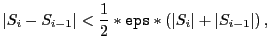
The eps parameter controls when the optimization will cease; for LEVENBERG-MARQUARDT, this will occur when
| (4.2) |
The smplx parameter controls whether the LEVENBERG-MARQUARDT fit
is refined with a SIMPLEX fit.
SIMPLEX refinement
can be useful for complicated fitting problems where straight
LEVENBERG-MARQUARDT does not provide a quick solution. Switchover from
LEVENBERG-MARQUARDT to
SIMPLEX occurs when ![]() ,
the change in statistic value from one iteration to the next, is
less than
LEVENBERG-MARQUARDT.smplxep, for
LEVENBERG-MARQUARDT.smplxit iterations in a row.
For example, the default is for switchover to occur when
,
the change in statistic value from one iteration to the next, is
less than
LEVENBERG-MARQUARDT.smplxep, for
LEVENBERG-MARQUARDT.smplxit iterations in a row.
For example, the default is for switchover to occur when
![]() 1 for 3 iterations in a row.
1 for 3 iterations in a row.
Parameters:
| Number | Name | Default | Min | Max | Description |
|---|---|---|---|---|---|
| 1 | iters | 2000 | 1 | 10000 | Maximum number of iterations. |
| 2 | eps | 1.e-3 | 1.e-9 | 1 | Criterion to stop fit. |
| 3 | smplx | 1 | 0 | 1 | Refine fit with simplex (0 |
| 4 | smplxep | 1 | 0.0001 | 1000 | Switch-to-simplex eps factor |
| 5 | smplxit | 3 | 1 | 20 | Switch-to-simplex iters factor |
A Monte Carlo search of parameter space.
The MONTECARLO method randomly samples the parameter space bounded by the lower and upper limits of each thawed parameter. At each chosen point, the fit statistic is evaluated. The advantage of MONTECARLO is that it can provide a good sampling of parameter space. This is good for situations where the best-fit parameter values are not easily guessed a priori, and where there is a high probability that false minima would be found if one-shot techniques such as POWELL are used instead. Its disadvantages are that it can be slow (if many points are selected), and that because of the random, discrete nature of the search, the global fit-statistic minimum can easily be missed. (The latter disadvantage may be alleviated by combining a Monte Carlo search with Powell minimization; see MONTE-POWELL.)
If the number of thawed parameters is larger than 3, one should increase the value of nloop from its default value. Otherwise the sampling may be too sparse to estimate the global fit-statistic minimum well.
Parameters:
| Number | Name | Default | Min | Max | Description |
|---|---|---|---|---|---|
| 1 | nloop | 500 | 1 | 1.6777e+7 | Number of parameter space samples. |
| 2 | iseed | 14391 | -1.e+20 | 1.e+20 | Seed for random number generator. |
A Monte Carlo search utilizing the Powell method at each selected point.
The MONTE-LM method randomly samples the parameter space bounded by the lower and upper limits for each thawed parameter. At each grid point, the LEVENBERG-MARQUARDT optimization method is used to determine the local fit-statistic minimum. The smallest of all observed minima is then adopted as the global fit-statistic minimum. The advantage of MONTE-LM is that it can provide a good sampling of parameter space. This is good for situations where the best-fit parameter values are not easily guessed a priori, and where there is a high probability that false minima would be found if one-shot techniques such as LEVENBERG-MARQUARDT are used instead. Its disadvantage is that it can be slow.
The MONTE-LM method parameters are a superset of those listed for the LEVENBERG-MARQUARDT method and the ones listed below.
If the number of thawed parameters is larger than 2, one should increase the value of nloop from its default value. Otherwise the sampling may be too sparse to estimate the global fit-statistic minimum well.
Parameters:
| Number | Name | Default | Min | Max | Description |
|---|---|---|---|---|---|
| 1 | nloop | 128 | 1 | 16384 | Number of parameter space samples. |
| 2 | iseed | 14391 | -1.e+20 | 1.e+20 | Seed for random number generator. |
A Monte Carlo search utilizing the Powell method at each selected point.
The MONTE-POWELL method randomly samples the parameter space bounded by the lower and upper limits for each thawed parameter. At each grid point, the POWELL optimization method is used to determine the local fit-statistic minimum. The smallest of all observed minima is then adopted as the global fit-statistic minimum. The advantage of MONTE-POWELL is that it can provide a good sampling of parameter space. This is good for situations where the best-fit parameter values are not easily guessed a priori, and where there is a high probability that false minima would be found if one-shot techniques such as POWELL are used instead. Its disadvantage is that it can be very slow.
Note that MONTE-POWELL is similar in nature to GRID-POWELL; in the latter method, the initial parameter values in each cycle are determined from a grid, rather than being chosen randomly.
The MONTE-POWELL method parameters are a superset of those listed for the POWELL method and the ones listed below.
If the number of thawed parameters is larger than 2, one should increase the value of nloop from its default value. Otherwise the sampling may be too sparse to estimate the global fit-statistic minimum well.
Parameters:
| Number | Name | Default | Min | Max | Description |
|---|---|---|---|---|---|
| 1 | nloop | 128 | 1 | 16384 | Number of parameter space samples. |
| 2 | iseed | 14391 | -1.e+20 | 1.e+20 | Seed for random number generator. |
The Powell optimization method.
The POWELL method is a single-shot method which attempts to find the local fit-statistic minimum nearest to the starting point. Its principal advantage is that it is a robust direction-set method. A set of directions (e.g., unit vectors) are defined; the method moves along one direction until a minimum is reached, then from there moves along the next direction until a minimum is reached, and so on, cycling through the whole set of directions until the fit statistic is minimized for a particular iteration. The set of directions is then updated and the algorithm proceeds. Its principal disadvantages are that it will not find the local minimum as quickly as LEVENBERG-MARQUARDT if the statistic surface is well-behaved, and there is no guarantee it will find the global fit-statistic minimum.
The eps parameter controls when the optimization will cease; for POWELL, this will occur when
 |
(4.3) |
Parameters:
| Number | Name | Default | Min | Max | Description |
|---|---|---|---|---|---|
| 1 | iters | 2000 | 1 | 10000 | Maximum number of iterations. |
| 2 | eps | 1.e-6 | 1.e-9 | 0.001 | Criterion to stop fit. |
| 3 | tol | 1.e-6 | 1.e-8 | 0.1 | Tolerance in lnmnop |
| 4 | huge | 1.e+10 | 1000 | 1.e+12 | Vestigial. |
The SIGMA-REJECTION optimization method for fits to 1-D data.
Abbreviated equivalents are SIG-REJ and SR.
The SIGMA-REJECTION optimization method is based upon the IRAF method SFIT. It iteratively fits data: a best-fit to the data is determined using a `regular' optimization method (e.g. LEVENBERG-MARQUARDT), then outliers data points are filtered out of the dataset, and the data refit, etc. Iterations cease when there is no change in the filter from one iteration to the next, or when the fit has iterated a user-specified maximum number of times.
Parameters:
| Number | Name | Default | Min | Max | Description |
|---|---|---|---|---|---|
| 1 | niter | 5 | 0 | 128 | The maximum number of iterations in the fit; if 0, the fit will run to convergence (i.e., until there is no change in the filter). |
| 2 | lrej | 3 | 0 | 10 | Data point rejection criterion in units of
|
| 3 | hrej | 3 | 0 | 10 | Data point rejection criterion in units of
|
| 4 | grow | 0 | 0 | 1024 | When a given data point is to be filtered out, this parameter sets the number of pixels adjacent to that pixel which are also to be filtered out, i.e., if 0, only the data point itself is filtered out; if 1, the data point and its two immediate neighbors are filtered out, etc. |
| 5 | omethod | lm | The optimization method to use to perform fits at each iteration. Note that quotes are required around the name! |
A simplex optimization method.
The SIMPLEX method is a single-shot method which attempts to find the local fit-statistic minimum nearest to the starting point. Its principal advantage is that it can work well with complicated statistic surfaces (more so than LEVENBERG-MARQUARDT), while also working quickly (more so than POWELL). Its principal disadvantages are that it has a tendency to "get stuck'' in regions with complicated topology before reaching the local fit-statistic minimum, and that there is no guarantee it will find the global fit-statistic minimum. Its tendency to stick means that the user may be best-served by repeating fits until the best-fit point does not change.
A simplex is geometrical form in ![]() -dimensional in parameter space
which has
-dimensional in parameter space
which has ![]() vertices (e.g.,
in 3-D it is a tetrahedron).
The fit statistic is evaluated for each vertex, and
one or more points of the simplex are moved, so that the simplex
moves towards the nearest local fit-statistic minimum.
When a minimum is reached, the simplex
may also contract itself, as an amoeba might; hence, the
routine is also sometimes called "amoeba.'' Convergence is
reached when the simplex settles into a minimum and all the
vertices are within some value eps of each other.
vertices (e.g.,
in 3-D it is a tetrahedron).
The fit statistic is evaluated for each vertex, and
one or more points of the simplex are moved, so that the simplex
moves towards the nearest local fit-statistic minimum.
When a minimum is reached, the simplex
may also contract itself, as an amoeba might; hence, the
routine is also sometimes called "amoeba.'' Convergence is
reached when the simplex settles into a minimum and all the
vertices are within some value eps of each other.
The eps parameter controls when the optimization will cease; for SIMPLEX, this will occur when
| (4.4) |
Parameters:
| Number | Name | Default | Min | Max | Description |
|---|---|---|---|---|---|
| 1 | iters | 2000 | 1 | 10000 | Maximum number of iterations. |
| 2 | eps | 1.e-6 | 1.e-9 | 0.001 | Criterion to stop fit. |
| 3 | alpha | 1 | 0.1 | 2 | Algorithm convergence factor. |
| 4 | beta | 0.5 | 0.05 | 1 | Algorithm convergence factor. |
| 5 | gamma | 2 | 1.1 | 20 | Algorithm convergence factor. |
A simulated annealing search, with one parameter varied at each step.
The SIMUL-ANN-1 method is a simulated annealing method. Such a method is said to be useful when a desired global minimum is among many other local minima. It has been derived via an analogy to how metals cool and anneal; as the liquid metal is cooled slowly, the atoms are able to settle into their minimum energy state, i.e. form a crystal. In simulated annealing, the function to be optimized is held to be the analog of energy, and the system slowly "cooled.'' At each temperature tried, the parameters are randomly varied; when there is no further improvement, the temperature is lowered, and again the parameters are varied some number of times. With sufficiently slow cooling, and sufficient random tries, the algorithm "freezes'' near the global minimum. (At each randomization, only one parameter is varied.) This is quite different from the other techniques implemented here, which can be said to head downhill, fast, for a nearby minimum. The great advantage of simulated annealing is that it sometimes goes uphill, thus escaping undesirable local minima the other techniques tend to get stuck in. The great disadvantage, of course, is that it is a slow technique.
A simple view of simulated annealing is that a new guess at the location of the minimum of the objective function is acceptable if it causes the value of the function to decrease, and also with probability
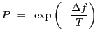 |
(4.5) |
where ![]() is the increase in the value of the objective
function, and T is a "temperature.'' After a large number of random
points in parameter space have been sampled, and no improvement in
the minimum value of the objective function has occurred, the
temperature is decreased (increasing the probability penalty for
positive
is the increase in the value of the objective
function, and T is a "temperature.'' After a large number of random
points in parameter space have been sampled, and no improvement in
the minimum value of the objective function has occurred, the
temperature is decreased (increasing the probability penalty for
positive ![]() ), and the process is repeated. The expectation is
that with a sufficient number of sampled points at each
temperature, and a sufficiently slow "cooling'' of the system, the
result will "freeze out'' at the true minimum. The analogy is
supposed to be with a cooling gas, where the Boltzmann statistics of
molecular motions causes the molecules of the gas to explore both the
minimum energy state and adjacent energy states at any one
temperature, and then freeze in a crystalline state of minimum energy
as the temperature approaches zero.
), and the process is repeated. The expectation is
that with a sufficient number of sampled points at each
temperature, and a sufficiently slow "cooling'' of the system, the
result will "freeze out'' at the true minimum. The analogy is
supposed to be with a cooling gas, where the Boltzmann statistics of
molecular motions causes the molecules of the gas to explore both the
minimum energy state and adjacent energy states at any one
temperature, and then freeze in a crystalline state of minimum energy
as the temperature approaches zero.
SIMUL-ANN-1 starts with a temperature which is about twice the initial value of the objective function, and reduces it slowly towards zero, changing a single parameter value at each randomization.
Parameter tchn is a multiplying factor for the temperature variable between cooling steps. Its default value of 0.98 means that a large number of cooling steps is needed to reduce the temperature sufficiently that the function "freezes out,'' but fast cooling is not recommended (as it inhibits the ergodic occupation of the search space). Parameter nloop specifies the maximum number of temperature values to try-but may be overridden if the code finds that the solution has "frozen out'' early. Finally, parameter nsamp specifies the number of movements at each temperature-the number of random changes to the parameter values that will be tried.
SIMUL-ANN-1 tends to be slow, but is a possible way of
making significant progress in traveling-salesman type problems.
One of its strengths is that even if it doesn't find the absolutely best
solution, it often converges to a solution that is close (in the
![]() sense) to the true minimum solution.
Somewhat better results are often obtained by SIMUL-POW-1
and SIMUL-POW-2,
where the
simulated annealing method is combined with the Powell method.
sense) to the true minimum solution.
Somewhat better results are often obtained by SIMUL-POW-1
and SIMUL-POW-2,
where the
simulated annealing method is combined with the Powell method.
Parameters:
| Number | Name | Default | Min | Max | Description |
|---|---|---|---|---|---|
| 1 | nloop | 512 | 32 | 8192 | Maximum number of temperatures. |
| 2 | tchn | 0.98 | 0.1 | 0.9999 | Factor for temperature reduction. |
| 3 | nsamp | 256 | 16 | 4096 | Number of movements at each temperature. |
| 4 | iseed | 14391 | -1.e+20 | 1.e+20 | Seed for random number generator. |
| 5 | tiny | 1.e-12 | 1.e-20 | 1.e-6 | Smallest temperature allowed. |
A simulated annealing search, with all parameters varied at each step.
The SIMUL-ANN-2 method is a simulated annealing method, analogous to SIMUL-ANN-1 in every way except that at each randomization, all the parameters are varied, not just one.
Note that the default temperature cycle change factor, and the number of temperature cycles, correspond to more and faster changes of temperature than SIMUL-ANN-1. This is because of the increased mobility within parameter space, since all values are changed with each randomization.
Parameters:
| Number | Name | Default | Min | Max | Description |
|---|---|---|---|---|---|
| 1 | nloop | 1024 | 64 | 16384 | Maximum number of temperatures. |
| 2 | tchn | 0.95 | 0.1 | 0.9999 | Factor for temperature reduction. |
| 3 | nsamp | 512 | 32 | 8192 | Number of movements at each temperature. |
| 4 | iseed | 14391 | -1.e+20 | 1.e+20 | Seed for random number generator. |
| 5 | tiny | 1.e-12 | 1.e-20 | 1.e-6 | Smallest temperature allowed. |
A combination of SIMUL-ANN-1 with POWELL.
This method packages together SIMUL-ANN-1 and the POWELL routine; at the end of each of the cooling sequences, or annealing cycles, the POWELL method is invoked. Probably one of the best choices where one `best' answer is to be found, but at the expense of a lot of computer time.
Note that the parameters of SIMUL-POW-1 are those of SIMUL-POW-1 itself (which have the same meaning as in routine SIMUL-ANN-1), plus those of POWELL.
All of the SIMUL-POW-1 parameters, with the exception of nanne, are explained under SIMUL-ANN-1. Parameter nanne specifies the number of annealing cycles to be used; successive anneal cycles start from cooler temperatures and have slower cooling. The pattern of anneals that has been chosen (the "annealing history'') is not magic in any way-for best results a different annealing history may be better for any particular objective function-but the pattern chosen seems to serve well.
Parameters:
| Number | Name | Default | Min | Max | Description |
|---|---|---|---|---|---|
| 1 | nloop | 256 | 16 | 4096 | Maximum number of temperatures. |
| 2 | tchn | 0.95 | 0.1 | 0.9999 | Factor for temperature reduction. |
| 3 | nanne | 16 | 1 | 256 | Number of anneals. |
| 4 | nsamp | 128 | 16 | 1024 | Number of movements at each temperature. |
| 5 | iseed | 14391 | -1.e+20 | 1.e+20 | Seed for random number generator. |
| 6 | tiny | 1.e-12 | 1.e-20 | 1.e-6 | Smallest temperature allowed. |
A combination of SIMUL-ANN-2 with POWELL.
This method packages together SIMUL-ANN-2 and the POWELL routine; at the end of each of the cooling sequences, or annealing cycles, the POWELL method is invoked. The rate of cooling in each anneal loop may be much faster than in simulated annealing alone. Probably one of the best choices where one `best' answer is to be found, but at the expense of a lot of computer time.
Note that the parameters of SIMUL-POW-2 are those of SIMUL-POW-2 itself (which have the same meaning as in routine SIMUL-ANN-2), plus those of POWELL.
All of the SIMUL-POW-2 parameters, with the exception of nanne, are explained under SIMUL-ANN-2. Parameter nanne specifies the number of annealing cycles to be used; successive anneal cycles start from cooler temperatures and have slower cooling. The pattern of anneals that has been chosen (the "annealing history'') is not magic in any way-for best results a different annealing history may be better for any particular objective function-but the pattern chosen seems to serve well.
Parameters:
| Number | Name | Default | Min | Max | Description |
|---|---|---|---|---|---|
| 1 | nloop | 256 | 16 | 4096 | Maximum number of temperatures. |
| 2 | tchn | 0.95 | 0.1 | 0.9999 | Factor for temperature reduction. |
| 3 | nanne | 16 | 1 | 256 | Number of anneals. |
| 4 | nsamp | 128 | 16 | 1024 | Number of movements at each temperature. |
| 5 | iseed | 14391 | -1.e+20 | 1.e+20 | Seed for random number generator. |
| 6 | tiny | 1.e-12 | 1.e-20 | 1.e-6 | Smallest temperature allowed. |
A user-defined method.
It is possible for the user to create and implement his or her own model, own optimization method, and own statistic function within Sherpa. The User Models, Statistics, and Methods Within Sherpa chapter of the Sherpa Reference Manual has more information on this topic.
The tar file sherpa_user.tar.gz contains the files needed to define the usermethod, e.g Makefiles and Implementation files, plus example files, and it is available from the Sherpa threads page: Data for Sherpa Threads
cxchelp@head.cfa.harvard.edu