HRC RMF

HRC-I | HRC-S | HRC/Cal

We have developed a new RMF for the HRC-I and HRC-S using scaled SUMAMPS (SAMP), rather than PHA, as a gain metric. Starting with CALDB 4.2/CIAO 4.2 (December 2009), PI will be calculated from SAMP instead of PHA. For more information about the gain maps used to convert SAMP to PI, see SUMAMPS-based Gain Maps for the HRC-I (Posson-Brown & Kashyap 2009) and A New Gain Map and Pulse-Height Filter for the Chandra LETG/HRC-S Spectrometer (Wargelin 2009).

This page discusses the creation of and justification for the RMF and provides grids in hardness-ratio space for some common spectral models, as calculated with the new RMF.

HRC-I

Introduction | Data and Analysis | Files | Grids

Vinay Kashyap & Jennifer Posson-Brown
December 2009

Introduction

The spectral resolution of the HRC-I is poor compared to the ACIS detectors, but it does exhibit a non-linear response to photon energies that can be advantageous in characterizing spectral hardness. To facilitate this, we have constructed a Redistribution Matrix file (RMF) that can be used in either Sherpa or XSPEC. A previous version of the RMF was constructed for use with 256-channel PI that was derived using PHA. Information about that RMF can be found here. The new version is for use with SAMP-derived 1024-channel PI values. For more information about the gain maps used to convert SAMP to PI, see Posson-Brown & Kashyap (2009).

Data and Analysis

First, we reprocess the data with hrc_process_events to apply the most recent calibration products. Next, we run CIAO tools (v4.1) tgdetect,tg_create_mask and tg_resolve_events on the event lists to assign a wavelength to each event based on its location. Finally, we use the SAMP-based gain maps to calculate PI for each event.

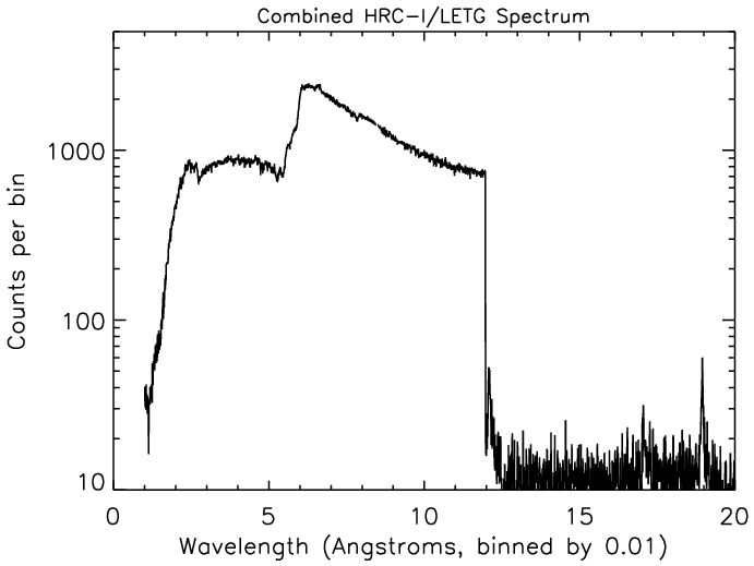
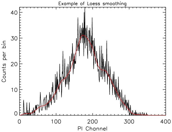
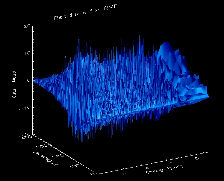
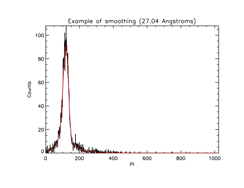
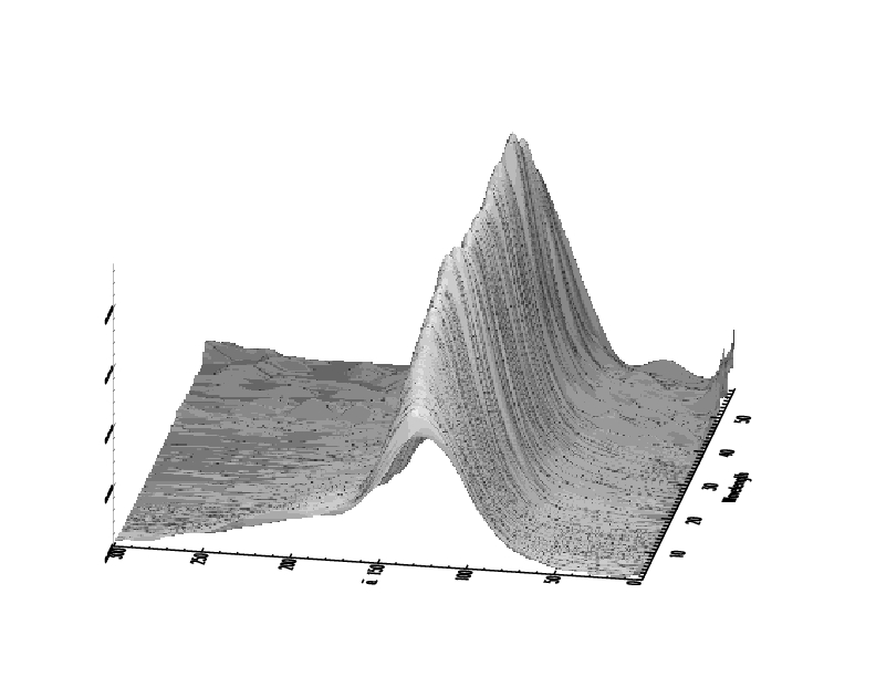
After filtering the data on the wavelength regions listed in Table 1, we combine the background-subtracted datasets, forming a two-dimensional PI/wavelength array. Figure 1 shows the combined spectrum (i.e. the two-dimensional array collapsed onto the wavelength axis). The array is then de-noised by carrying out polynomial fits over a moving window (Loess-type smoothing) along first the PI axis for a slice of wavelengths (over a wavelength range large enough to include 4000 counts in each slice), and then along the wavelength axis for each PI. Figure 2 shows an example of the data along a constant wavelength slice (~7.5 Angstroms) with the polynomial smoothing overplotted in red. Figure 3 shows the residuals between the data array and the smoothed array. The residuals are about +/- 20 counts at most, following with the general shape of the PI spectra, and there aren't any obvious features.

Figure 1: Combined HRC-I/LETG spectrum

Figure 2: Example of smoothing

Figure 3: Residuals

Files

• Gain correction maps are needed to remove the spatial dependence of the gain variations across the HRC-I and to account for the gain drop since Oct 99. As of CALDB 4.2, the default gain maps calculate PI from scaled SUMAMPS (Posson-Brown & Kashyap, 2009).

  For observations carried out at the high-voltage setting, i.e., prior to 1999-oct-04:

  $CALDB/data/chandra/hrc/gmap/hrciD1998-10-30sampgainN0001.fits

  For observations carried out after the change to lower-voltage setting, i.e., after 1999-oct-04:

  $CALDB/data/chandra/hrc/gmap/hrciD1999-10-04sampgainN0001.fits

  $CALDB/data/chandra/hrc/gmap/hrciD2000-12-12sampgainN0001.fits

  $CALDB/data/chandra/hrc/gmap/hrciD2002-01-26sampgainN0001.fits

  $CALDB/data/chandra/hrc/gmap/hrciD2003-02-22sampgainN0001.fits

  $CALDB/data/chandra/hrc/gmap/hrciD2004-11-25sampgainN0001.fits

  $CALDB/data/chandra/hrc/gmap/hrciD2005-10-17sampgainN0001.fits

  $CALDB/data/chandra/hrc/gmap/hrciD2006-09-20sampgainN0001.fits

  $CALDB/data/chandra/hrc/gmap/hrciD2007-09-17sampgainN0001.fits

  $CALDB/data/chandra/hrc//gmap/hrciD2008-09-07sampgainN0001.fits

  $CALDB/data/chandra/hrc//gmap/hrciD2009-09-24sampgainN0001.fits

  Note: A series of AR Lac observations were carried out at multiple voltage settings, at various locations on the detector, on 1999-oct-04. To compute PI values for these observations, the appropriate gain file must be set manually during a run of hrc_process_events.

   

• Version 1 of the new Response Matrix file for SAMP-based PI (available in CALDB 4.2):

  $CALDB/data/chandra/hrc/cpf/rmf/hrciD1999-07-22samprmfN0001.fits

  WARNING: Do not use for spectral fits; the spectral response is not sufficiently constraining to achieve a good fit with reasonable errors. If unavoidable, work in channel space (setplot channel in XSPEC or set_analysis("chan") in Sherpa), not in energy space.

   

Grids

In Figures 4-7 we provide grids in hardness-ratio space for some common spectral models, as calculated using the HRC-I RMF derived above and a nominal on-axis ARF. The grids were calculated using Sherpa. For the hardness ratio, we choose three bands in PI,

S == 50:130

M == 131:200

H == 201:280

C_SM=log₁₀(S/M) and

C_MH=log₁₀(M/H).

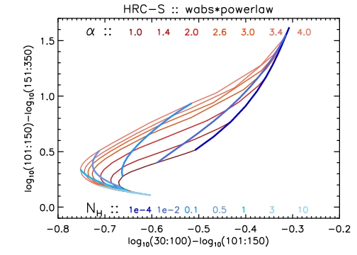
Figure 4: Color-color grid for powerlaw model

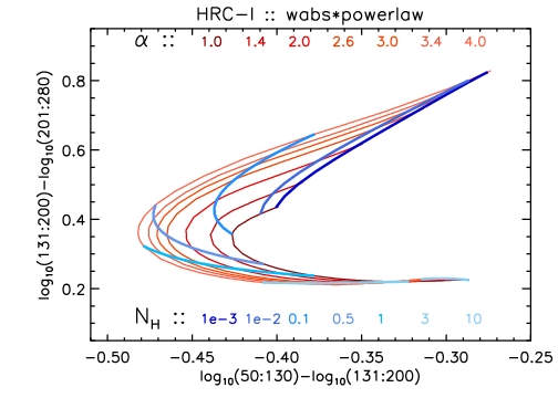
The color-color grid for a powerlaw model, calculated for various values of the powerlaw index Gamma (red loci) and absorption column N_H [10²² cm^-2] (blue loci).

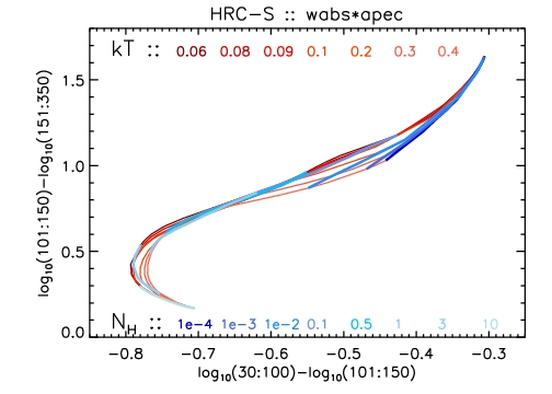
Figure 5: Color-color grid for low temperature APEC model

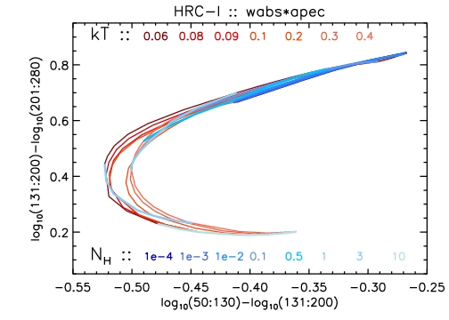
The color-color grid for an APEC model, calculated for relatively low values of the plasma temperature kT [keV] (red loci) and absorption column N_H [10²² cm^-2] (blue loci).

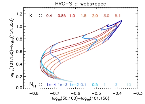
Figure 6: Color-color grid for high temperature APEC model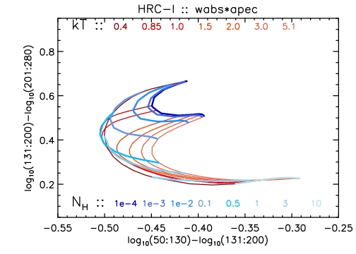

The color-color grid for an APEC model, calculated for relatively high values of the plasma temperature kT [keV] (red loci) and absorption column N_H [10²² cm^-2] (blue loci).

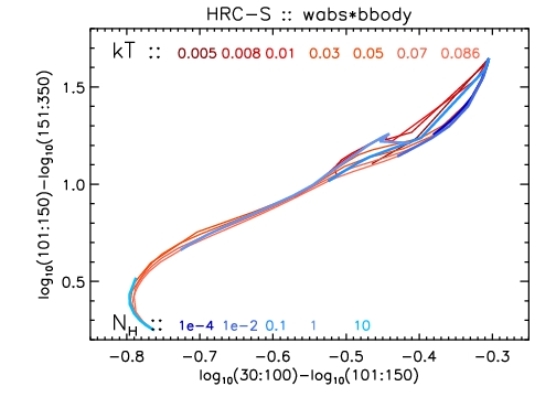
Figure 7: Color-color grid for blackbody model

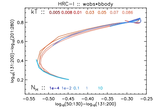
The color-color grid for a Blackbody model, calculated for various values of the temperature kT [keV] (red loci) and absorption column N_H [10²² cm^-2] (blue loci).

References

• Kashyap V & Posson-Brown J, 2009, Proc. of the 2009 Chandra Calibration Review
  http://cxc.harvard.edu/ccr/proceedings/2009/presentations/kashyap/
• Park T Y, Kashyap V, Zezas A, Siemiginowska A, van Dyk D, Connors A & Heinke C, 2006, ApJ, 652, 610
  http://hea-www.harvard.edu/AstroStat/BEHR/
• Posson-Brown J. & Kashyap V., 2009, "SUMAMPS-based Gain Maps for the HRC-I"
  http://cxc.harvard.edu/cal/Hrc/Documents/Gain/hrci_sampgain_nov2009.pdf

Introduction | Data and Analysis | Files | Grids

Vinay Kashyap & Jennifer Posson-Brown
October 2010

Introduction

The spectral resolution of the HRC-S in imaging mode is poor compared to that of the ACIS detectors, but the HRC-S does exhibit a non-linear response to photon energies that can be advantageous in characterizing spectral hardness. To facilitate this, we have constructed a Redistribution Matrix file (RMF) that can be used in either Sherpa or XSPEC. A previous version of the RMF was constructed for use with 256-channel PI that was derived using PHA. Information about that RMF can be found here. The new version is for use with SAMP-derived 1024-channel PI values. For more information about the gain map used to convert SAMP to PI, see HRC-S Gain Map and LETG Background Filter.

Data and Analysis

First, we reprocess the data with hrc_process_events (CIAO v4.2, CALDB v4.2) to apply the most recent calibration products, including the time-dependent gain correction which converts scaled-SUMAMPS to PI. We then run tgdetect,tg_create_mask and tg_resolve_events on the event lists to assign a wavelength to each event based on its location.

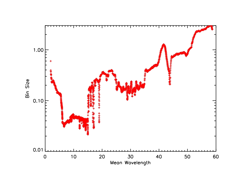
After filtering the data on the wavelength regions listed in Table 1, we bin the data in wavelength to have approximately 4000 counts per bin after background subtraction. The resulting bin sizes range from ~0.02 to ~1.2 Angstroms, see Figure 1. We then form two-dimensional PI/wavelength arrays for source and background using these wavelength bins and 1 channel PI bins.

Next, the source and background arrays are Loess-smoothed, first along PI for each wavelength bin then along wavelength for each PI bin. An example of this smoothing is shown in Figure 2. We then subtracted the smoothed background array (multiplied by extraction area ratio) from the smoothed source array. Finally, we normalize this net array so that the sum over each wavelength bin is 1. The resulting RMF is shown in Figure 3.

Figure 1: Bin size (Angstroms) as a function of wavelength, to get 4000 cts/bin

Figure 2: Example of Loess smoothing

Figure 3: RMF

Files

• The gain correction map is needed to remove the spatial and time dependence of the gain variations across the HRC-S and generate PI values mimicking an on-axis observation. This map is available in the CALDB (see the HRC-S Gain Map and LETG Background Filter for details).

  $CALDB/data/chandra/hrc/t_gmap/hrcsD1999-07-22t_gmapN0001.fits

   

• Version 1 of the Response Matrix file (available in CALDB 4.3):

  $CALDB/data/chandra/hrc/rmf/hrcsD1999-07-22samprmfN0001.fits

  WARNING: Do not use for spectral fits; the spectral response is not sufficiently constraining to achieve a good fit with reasonable errors. Work should be conducted in channel space (setplot channel in XSPEC or set_analysis("chan") in Sherpa), not energy space. The correspondence between PI bins and energy values is not well-defined.

   

Grids

Here we provide hardness-ratio grids for some common spectral models, calculated using the HRC-S RMF derived above and a nominal on-axis ARF. The grids were calculated using Sherpa. For the hardness ratio, we choose three bands in PI,

S == 30:100

M == 101:150

H == 151:350

C_SM=log₁₀(S/M) and

C_MH=log₁₀(M/H).

References

• HRC-S Gain Map and LETG Background Filter [LETG Calibration Group]
• Park T Y, Kashyap V, Zezas A, Siemiginowska A, van Dyk D, Connors A & Heinke C, 2006, ApJ, 652, 610
  http://hea-www.harvard.edu/AstroStat/BEHR/
• Wargelin, B, 2009, Proc. of the 2009 Chandra Calibration Review
  http://cxc.harvard.edu/ccr/proceedings/2009/presentations/wargelin/

Last modified: 11/18/13

The Chandra X-Ray Center (CXC) is operated for NASA by the Smithsonian Astrophysical Observatory. 60 Garden Street, Cambridge, MA 02138 USA.    Email: cxcweb@head.cfa.harvard.edu Smithsonian Institution, Copyright © 1998-2004. All rights reserved.