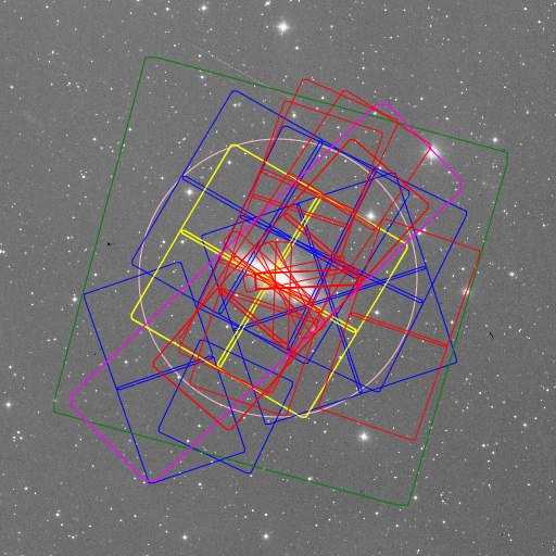
I review the contribution of Chandra X-ray Observatory to studies of dark energy. There are two broad classes of observable effects of dark energy: evolution of the expansion rate of the Universe, and slow-down in the rate of growth of cosmic structures. Chandra has detected and measured both of these effects through observations of galaxy clusters. Combination of the Chandra results with other cosmological datasets leads to 5% constraints on the dark energy equation-of-state parameter, and limits possible deviations of gravity on large scales from General Relativity.
Introduction
The accelerated expansion of the Universe discovered in 1998 [1, 2] and the associated problem of dark energy are widely considered as one of the greatest unsolved problems in science. In this short article, I will summarize the contribution of X-ray astronomy (primarily, Chandra and XMM-Newton) to the currently emerging picture of empirical properties of dark energy.
There are two main observable manifestations of dark energy. The first is its effect on the expansion rate of the Universe as a whole, which can be probed through the distance-redshift relation using “standard candles” such as type Ia supernovae, or standard rulers such as baryonic acoustic oscillations in the large-scale distribution of galaxies [3]. This broad class of cosmological observations is often referred to as “geometric” methods. The second effect is the impact of dark energy on the rate of growth of large-scale structures. As the Universe enters the accelerated expansion phase around z ~ 0.8, it is expected that the rate of structure growth slows down. If this effect is observed sufficiently accurately – e.g., through weak lensing on the large-scale structures, redshift-space distortions in the distribution of galaxies [4], or through evolution of galaxy clusters as described below – it should significantly improve constraints on dark energy properties in combination with the geometric methods [3]. In addition, the growth of large-scale structures can be used to test, or put limits on, any departures from General Relativity on the 10—100 Mpc scales [5].
X-ray astronomy's contribution to observational cosmology is primarily through studies of galaxy clusters. Cluster observations provide both the geometrical and growth of structure cosmological tests. The distance-redshift relation can be measured either through the Sunyaev-Zel'dovich [6] effect, or using the expected universality of the intracluster gas mass fraction, fgas = Mgas/Mtot [7,8]. Both methods can also be used to determine the absolute value of the Hubble constant through observations of low-z clusters1. The mass function of galaxy clusters is exponentially sensitive to the underlying amplitude of linear density perturbations and therefore can be used to implement the growth of structure test [11].
In the Chandra and XMM-Newton era,
X-ray observations of galaxy clusters
have reached sufficient maturity for a
successful implementation of both
types of cosmological tests. This
success is based on significant
advances in our ability to select and
statistically characterize large
cluster samples, and to get detailed
X-ray data at both low and high
redshifts. At the same time, quick
progress in theoretical modeling of
clusters (see [12] for a recent
review) resulted in better
understanding of their physics and
improved ability to obtain reliable
mass estimates from the data. These
advances are reviewed below.
Combining the Sunyaev-Zel'dovich effect observations and X-ray data for the same cluster naturally provides the absolute distance to the object [9]. In the gas fraction method, it is assumed that the baryon mass fraction within clusters, fb, approximates the mean cosmic value, Ωb//Ωm. The absolute value of this ratio is now very well known from the CMB data [10]. On the other hand, the mass fraction of the hot intracluster gas, the dominant baryonic component in clusters, derived from the X-ray data is proportional to h-3/2 (see below in the text), therefore h can be extracted from these measurements after correcting fgas for the contribution of stellar mass to the total baryon budget.
Progress in understanding of clusters
Samples
The ROSAT mission which operated in the 1990s proved to be a great resource for selecting large, complete samples of massive galaxy clusters reaching redshifts beyond z=1 [13]. ROSAT carried out surveys in a wide range of sensitivity and solid angle. The sensitivity and angular resolution in the all-sky survey mode are well-suited for detection of clusters at low redshifts (e.g., the BCS and REFLEX surveys, [14, 15]). With substantial effort on the optical identification side, the all-sky survey data can be used to select exceptionally massive clusters out to z ~ 0.5 (MACS survey, [16]). In the pointed mode, ROSAT PSPC covered just over 2% of the extragalactic sky. However, the sensitivity and angular resolution in the pointed mode are sufficient for detection of z ~ 0.6 clusters with masses matching those of the low-z objects detected in the all-sky survey. Just such a sample of clusters is provided by the 400d survey [17]. The REFLEX, MACS, and 400d surveys, several hundred clusters each, are the main sources for cosmological observations with Chandra.
Detailed Measurements
Chandra and XMM-Newton observations of low-redshift objects now provide detailed measurements of the radial profiles of the density, temperature, and metallicity of the intracluster medium (ICM) over a wide range of radii. Several studies (Chandra samples of high-mass relaxed clusters [18]; Chandra studies of low-M groups [19]; XMM-Newton representative cluster samples [20] including both relaxed and unrelaxed objects) provide a consistent picture. The gas density and temperature profiles show a high degree of regularity and follow simple scalings outside the inner cluster region (Figures 1 and 2). At large radii, the observed scaling of the ICM entropy with cluster mass is close to that predicted for purely gravitational heating [21, 22]. However, deviations from such a scaling are observed at small radii, indicating more complex physics in the inner cluster region. Such measurements are important for cosmological applications of the cluster data for several reasons. First, they provide the necessary observational ingredients for estimation of the cluster total masses via the hydrostatic equilibrium equation. Second, the observed ICM profiles can be used to verify numerical models of the cluster formation [21]. The main role of numerical models in the cosmological applications of the cluster data is to provide predictions for the scaling relations between total mass and global X-ray properties. These predictions can be used reliably only because we can verify that numerical models reasonably well reproduce even more complex cluster properties. Last, self-similarity of the observed ICM profiles directly demonstrates that the cluster properties are predominantly determined by a single parameter, its mass. This is a key notion in the theory of cluster formation, and the basis for using clusters as cosmological probes.
Mass Measurements
The existence of scaling relations between various cluster parameters and total mass has long been recognized. However, establishing the absolute scale in such relations is a long-standing problem. The situation today is much improved. A good agreement, at a ~ 10% level in mass, exists [23] between normalizations of the mass vs. proxy relations determined from the X-ray measurements in relaxed clusters (e.g., [18]), “measured” in numerical simulations [24, 25], and obtained from weak lensing observations of representative samples of intermediate redshift clusters [26, 27]. A 10% accuracy in the absolute cluster mass calibration is indicated not only by the agreement of the results from different methods, but also indirectly by agreement of the amplitude of density perturbations derived from X-ray clusters [28], from optically selected clusters with masses calibrated through weak lensing [29], and from the latest weak lensing shear studies [30].
The advances in theoretical and
observational studies of galaxy
clusters outlined above, which were
triggered in large part by the Chandra
and XMM-Newton observations, have
enabled efficient application of the
geometrical and structure-based
cosmological tests.
Figure 1: Scaled total and gas density profiles measured in
a sample of high-mass relaxed clusters observed with Chandra
(reproduced from [18]). To properly compare clusters at
different redshifts and with different masses, the densities
were scaled by ρc(z), the critical density at the
object's redshift, and the radii were scaled by r500
– the radius within which the mean density is 500
ρc(z).
Geometric test with fgas
Galaxy clusters are expected to have a nearly cosmic mix of baryonic and dark matter, fb = Mb/Mtot ≈ Ωb/ΩM, because their mass is orders of magnitude higher than the Jeans mass scale and hence baryons and dark matter are not separated as the clusters grow from large-scale structures [31]. The universality of the baryon fraction in clusters was originally used as a method for measuring ΩM, but in the mid-1990's it was realized that it can be also used as an independent distance indicator [7, 8]. The mass of the intracluster gas (contributing 80%—90% to the total baryonic mass in massive clusters [32]) derived from the X-ray image is proportional to d5/2 where d is the distance to the cluster, while dynamically-derived total mass scales as d1. Therefore, the apparent baryon mass fraction is proportional to 33/2 and is constant as a function of z only if we use the correct distance-redshift relation.
Early pilot studies based on this test were inconclusive [8, 33]. Comparison of the Chandra results [34] with these early works exemplifies just how revolutionary Chandra has been for cluster cosmology (Figure 3). The object-to-object scatter is now low and the trends in the fgas(z) data arising from assuming a “wrong” cosmological model are clearly detectable. In particular, the expected absence of redshift trends in the fgas measurements is only for the range of parameters corresponding to the “concordant” cosmological models, while strong trends in fgas (z) are found if, e.g., one assumes an ΩM= 1 model without a cosmological constant [34].
Unfortunately, the assumption that
fgas (and even the total baryon
fraction including stellar mass) in
clusters is constant and universal is
only approximately accurate because
there are observed trends with radius
within individual clusters. The fgas
values measured at a fixed fraction of
the virial radius also show a trend
with cluster mass [18, 19, 22]. The
nature of these trends remains
uncertain. Feasible explanations
include different star formation
efficiencies in high and low-mass
clusters, and some form of
non-gravitational heating of the gas
in the central regions. Existence of
fgas trends in the low-z clusters
almost certainly implies that fgas
should slightly vary with
redshift. Allen et al. [34] corrected
for some of these effects using
results from numerical
simulations. Unfortunately,
non-negligible systematic
uncertainties must be assigned (e.g.,
Allen et al. allowed for ± 10%
variations of intrinsic fgas between
z=0 and 1), and they dominate the
final error budget when the fgas test
is used, for example, to constrain the
dark energy equation-of-state
parameter, w. Even with the current
level of systematic uncertainties, the
fgas test provides interesting
constraints on the value of w (Figure
4).
Figure 2: Scaled temperature profiles from a representative cluster sample observed with XMM-Newton (reproduced from [20]). The temperature profiles are scaled to the average temperature for each cluster, and the radii are scaled to the critical overdensity radius r200.
Growth of structure test
Evolution of the cluster mass function traces (with exponential magnification) the growth of linear density perturbations. Growth of structure and the distance-redshift relation are similarly sensitive to properties of dark energy, and also are highly complementary sources of cosmological information (e.g., [35]). Pre-Chandra studies using the cluster mass function as a cosmological probe were limited by small sample sizes. They also had to use either poor proxies for the total mass (e.g., the X-ray flux) or inaccurate measurements (e.g., temperatures with large uncertainties). Despite these limitations, reasonable constraints could still be derived on Ωm (e.g., [36, 37]). However, constraints on the dark energy equation-of-state parameter from such studies were weak.
As discussed above, the situation with the cluster mass function data has dramatically improved in the past three years, and the new measurements allow us to track the growth of density perturbations over the redshift interval z=0-0.7. These measurements confirm the slow-down of that growth caused by cosmic acceleration, improve constraints on the equation-of-state parameter, and even put limits on possible departures from General Relativity on ~10 Mpc scales.
The sensitivity of the cluster mass function to the presence of dark energy is illustrated in Figure 5. The cluster sample used in [28] provides sufficient statistics to measure the amplitude of density perturbations independently in the redshift intervals z=0.015-0.15, 0.35-0.45, 0.45-0.55, and 0.55-0.9. Together with the amplitude of perturbations at z ~1000 derived from the cosmic microwave background fluctuations, these data track the growth of perturbations over a wide redshift interval (Figure 6). The slowdown of the perturbations growth at low redshifts is clearly seen, and the data indicate that the transition from fast to slow growth was fast and occurred at z ~ 1, as expected for models with dark energy (see, e.g., the solid red line in Figure 6 and compare it with the growth histories for low-density models without dark energy shown by blue dashed lines).
The evolution of the cluster mass
function measured from the 400d survey
provides sufficient statistics to
constrain the dark energy
equation-of-state parameter (Figure
7). The combination of the structure
growth data with other cosmological
datasets results, as was long
anticipated, in dramatic improvement
of the constraints. For example, a
non-evolving equation-of-state
parameter is constrained to be w0 =
-0.99 ± 0.045 (inner ellipse in
Figure 7); without the cluster data,
the statistical and systematic
uncertainties on w0 are a factor of
1.5-2 worse [28].
Figure 3: Implementation of the fgas(z) cosmological test using ROSAT and ASCA data (left, [33]), and with Chandra (right, [34]). The gas fractions in these two studies were derived assuming different values of H0, which explains an offset between average values for low-z clusters in the two panels. Chandra results are shown for the concordance ΛCDM cosmology; in the q0 = 0.5 model, for example, there would be a strong, easily detectable trend (e.g., Fig. 2b in [34]).
Figure 4: Constraints on the dark energy equation-of-state parameter, w, from the fgas(z) test and other cosmological datasets (reproduced from [34].
Testing non-GR models
Perhaps a more interesting application of the cluster mass function is to test for possible deviations from General Relativity on ~10 Mpc scales. Non-GR gravity theories modify the distance-redshift relations. However, the changes in d(z) generally can be mimicked by variations of the equation-of-state parameter for “true” dark energy and therefore non-GR models cannot be tested by geometric methods alone. We can test them using a combination of geometric measurements with the growth of structure data. Each of the essential ingredients of the cluster mass function theory – the growth of linear density perturbations, non-linear collapse of large-amplitude perturbations, and relations between the cluster mass and its observed properties – is potentially modified in non-GR gravity models.
Unfortunately, self-consistent predictions for the properties of the cluster population in non-GR models are still rare. Usually, the published analyses are restricted to predicted modifications of the structure growth rate in the linear regime. It has been suggested [5] that a useful parametrization for such deviations is the linear growth index, γ, defined as
D = (1+ z) exp [ - ∫∞z (ΩM(z)γ - 1) d ln (1 + z) ]
where D is the perturbations growth factor at redshift z. If D is measured at a set of redshifts, γ can be constrained by fitting the model curves given by eq. (1) to the data. The test is useful because it was found that for a wide range of models in which dark energy is represented by some form of a scalar field, γ ≈ 0.55 with high precision [5]. Therefore, if γ is found to significantly deviate from 0.55, this potentially would imply that gravity does not follow GR on the cluster scales. Unfortunately, implementations of this method using cluster data necessarily ignore potential effects of non-GR gravity on the non-linear collapse and relations between the cluster mass and observables. However, γ derived from the cluster data still provides a useful null test. The best published results from the X-ray cluster mass function constrain the growth index to be γ =0.44±0.16 [38]; no other cosmological test currently provides useful constraints on γ.
As of this writing, the only self-consistent test of a non-GR theory with the cluster data is presented by Schmidt et al. [39]. They consider a specific variant of a so-called f(R) models, in which two terms are added to the GR Lagrangian, one corresponding to Einstein's cosmological constant and another to a genuine modification of GR,
16 π Lg = R + f(R) = R - 16πGρΛ- fRR02/R
is the average present-day curvature in the Universe, and f(R) characterizes the fractional (with respect to R) modification of the Lagrangian density of the gravitational field. Schmidt et al. showed that a combination of the 400d survey cluster data with other cosmological datasets constrains the non-GR term to be f(R) < 10-3.
Figure 5: Illustration of sensitivity of the cluster mass function to the cosmological model. Following the usual convention (e.g. [40]), the masses are defined at the radius within which the mean cluster density is a factor of 500 higher than the critical density at that redshift M500 = Mtot(r500) where r500 is found from the condition Δcrit = Mtot(r500)/(4/3 π r5003ρc(z)) = 500). In the left panel, we show the measured mass function and predicted models (with only the overall normalization at z = 0 adjusted) computed for a cosmology which is close to our best-fit model. In the right panel, both the data and the models are computed for a cosmology with ΩΛ = 0. Both the model and the data at high redshifts are changed relative to the ΩΛ = 0.75 case. The measured mass function is changed because it is derived for a different distance-redshift relation. The model is changed because the predicted growth of structure and overdensity thresholds corresponding to Δcrit = 500 are different. When the overall model normalization is adjusted to the low-z mass function, the predicted number density of z > 0.55 clusters is in strong disagreement with the data, and therefore this combination of ΩM and ΩΛ can be rejected.
Figure 6: Normalized linear density perturbations amplitude derived from the 400d survey cluster sample (solid points). The amplitude is normalized to the initial amplitude at z ≈ 1000 measured by WMAP (open point, arbitrarily placed at z =4.5) and to the growth expected in an ΩM=1 universe without dark energy. Solid curve shows the growth expected in the concordance ΛCDM cosmology. Dashed lines shows the growth expected in models without dark energy, for different values of the ΩM parameter.
Figure 7: Constraints on the dark energy equation-of-state parameter from the growth of structure test with X-ray clusters, and from other cosmological datasets. The combination of methods (inner ellipse) gives w0= -0.991 ± 0.045 (±0.04 systematic) and ΩX = 0.740 ± .012 [28].
Conclusions
X-ray observations of massive galaxy clusters with Chandra and XMM-Newton have afforded robust implementations of the geometric and growth of structure cosmological tests. Cluster data independently confirm the accelerated expansion of the universe, show that the empirical properties of dark energy are very close to those of the cosmological constant, and start to provide interesting constraints on possible deviations of gravity from General Relativity on large scales.
References
[1] Riess, A. G., et al. (1998). AJ 116:1009–1038.
[2] Perlmutter, S., et al. (1999). ApJ 517:565–586.
[3] Albrecht, A., et al. (2006). astro-ph/0609591.
[4] Guzzo, L., et al. (2008). Nature 451:541–544.
[5] Huterer, D. & Linder, E. V. (2007). Phys. Rev. D 75:023519.
[6] Sunyaev, R. A. & Zeldovich, Y. B. (1972). Com. on Astroph. & Sp. Phys. 4:173.
[7] Sasaki, S. (1996). PASJ 48:L119–L122.
[8] Pen, U. (1997). New Astronomy 2:309–317.
[9] Silk, J. & White, S. D. M. (1978). ApJ 226:L103–L106.
[10] Dunkley, J., et al. (2009). ApJ Suppl 180:306–329.
[11] Oukbir, J. & Blanchard, A. (1992). A&A 262:L21–L24.
[12] Borgani, S. & Kravtsov, A. (2009). ArXiv:0906.4370.
[13] Rosati, P., Borgani, S., & Norman, C. (2002). Annual Reviews Astron. & Astrophys. 40:539–577.
[14] Ebeling, H., et al. (2000). MNRAS 318:333–340.
[15] Böhringer, H., et al. (2004). A&A 425:367–383.
[16] Ebeling, H., Edge, A. C., & Henry, J. P. (2001). ApJ 553:668–676.
[17] Burenin, R. A., et al. (2007). ApJ Suppl 172:561–582.
[18] Vikhlinin, A., et al. (2006). ApJ 640:691–709. (V06).
[19] Sun, M., et al. (2009). ApJ 693:1142–1172.
[20] Pratt, G. W., et al. (2007). A&A 461:71–80.
[21] Nagai, D., Kravtsov, A. V., & Vikhlinin, A. (2007). ApJ 668:1–14.
[22] Pratt, G. W., et al. (2010). A&A 511:A85+.
[23] Henry, J. P., Evrard, A. E., Hoekstra, H., Babul, A., & Mahdavi, A. (2009). ApJ 691:1307–1321.
[24] Rasia, E., et al. (2006). MNRAS 369:2013–2024.
[25] Nagai, D., Vikhlinin, A., & Kravtsov, A. V. (2007). ApJ 655:98–108.
[26] Hoekstra, H. (2007). MNRAS 379:317–330.
[27] Zhang, Y.-Y., et al. (2008). A&A 482:451–472.
[28] Vikhlinin, A., et al. (2009). ApJ 692:1060–1074.
[29] Rozo, E., et al. (2009). ArXiv e-prints.
[30] Fu, L., et al. (2008). A&A 479:9–25.
[31] White, S. D. M., Navarro, J. F., Evrard, A. E., & Frenk, C. S. (1993). Nature 366:429–433.
[32] Gonzalez, A. H., Zaritsky, D., & Zabludoff, A. I. (2007). ApJ 666:147–155.
[33] Rines, K., Forman, W., Pen, U., Jones, C., & Burg, R. (1999). ApJ 517:70–77.
[34] Allen, S. W., et al. (2008). MNRAS 383:879–896.
[35] Linder, E. V. & Jenkins, A. (2003). MNRAS 346:573–583.
[36] Borgani, S., et al. (2001). ApJ 561:13–21.
[37] Henry, J. P. (2004). ApJ 609:603–616.
[38] Rapetti, D., Allen, S. W., Mantz, A., & Ebeling, H. (2009). MNRAS 400:699–704.
[39] Schmidt, F., Vikhlinin, A., & Hu, W. (2009). Phys. Rev. D 80:083505.
[40] Evrard, A. E., et al. (2002). ApJ 573:7–36.
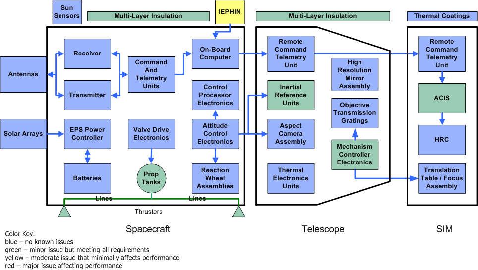
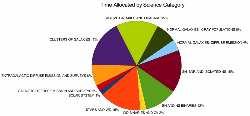
Project Scientist's Report
Martin Weisskopf
The marvel of Chandra exceeding its nominal operational life continues. The Observatory is now in its 12th year of successful operation, and the call for the 13th Cycle of proposals has been issued. Considering the implications of the most recent Decadal Survey of Astronomy and Astrophysics, we realize just how much the community needs the high-resolution of Chandra to accomplish its science. Moreover, the Observatory continues to operate with only minor incremental changes in performance, due primarily to slow degradation of the thermal insulation and to the gradual accumulation of molecular contamination on the ACIS filter. The former mainly impacts observing strategies and efficiencies so that we may operate the Observatory in a safe thermal environment. The latter has an impact for the detection of the softest x-rays with ACIS.
A major Project activity of the past year was to undergo the biennial NASA Senior Review of Operating Missions. As the largest program under review, the Chandra mission was under a lot of scrutiny. Thanks to the efforts of many dedicated people, to excellent presentations (by Harvey Tananbaum, Belinda Wilkes and Roger Brissenden), and to the science that the Observatory fosters, the Project came out with the (just next to) highest marks. The Senior Review even recommended some relief in projected spending cuts.
We have sponsored Chandra-focused symposia every two years for many years. This year we are doing something slightly different: We are sponsoring a “Meeting in a Meeting” (MiM) at the 218th AAS Meeting, in Boston, 2011 May. The Chandra MiM, “12 Years of Science with Chandra”, will comprise poster sessions and six 90-min sessions of invited talks. We encourage you to contribute a poster (see http://cxc.harvard.edu/symposium_2011/) and to attend the invited talks.
The oral sessions are:
Session 1 (05/23/2011, 10am-11:30am)
Title: What Chandra tells us about Solar System Objects
15-minute talk 1: Martin. C. Weisskopf, “The Chandra X-ray Observatory: Current Status and Future Prospects”
30-minute talk 1: Graziella Branduardi-Raymont, “High-Resolution Observations of Solar-System Objects”
30-minute talk 2: Brad Wargelin, “Covering Solar-Wind Charge Exchange from Every Angle with Chandra”
15-minute talk 2: Konrad Dennerl: “X-rays from Planetary Exospheres”
Session 2 (05/23/2011, 2pm-3:30pm)
Title: What Chandra tells us about Stars
30-minute talk 1: Manuel Guedel, “The X-ray Life of Stars”
15-minute talk 1: Joel Kastner, “Shaping Outflows from Evolved Stars: Secrets Revealed by Chandra”
15-minute talk 2: Jeremy Drake, “Swanning Around with Chandra: Star and Planet Formation in Cygnus OB2”
30-minute talk 2: Mike Corcoran, “X-ray Line Diagnostics of Shocked Outflows in Eta Carinae and Other Massive Stars”
Session 3: (05/24/2011, 10am-11:30am)
Title: What Chandra tells about SNR and Compact Objects
30-minute talk 1: Una Hwang, “A Million-Second Chandra View of Cassiopeia A”
30-minute talk 2: Edward Cackett, “Search for relativistic Fe lines in Chandra spectra of NS and BH LMXBs”
15-minute talk 1: Patrick Slane, “Using Chandra to constrain particle spectra in pulsar wind nebulae.”
15-minute talk 2: Joseph Neilsen, “GRS 1915+105: X-ray spectroscopic study of outflows”
Session 4 (05/24/2011, 2pm-3:30pm)
Title: What Chandra tells us about Galaxies
30-minute talk 1: Tom Maccarone, “Compact Object Formation in Globular Clusters, the Milky Way, and External Galaxies”
15-minute talk 1: Bret Lehmer, “X-ray emission from high-redshift star forming galaxies, results from the Chandra Deep Field South 4 Ms survey”
15-minute talk 2: K.D. Kuntz, “New ultra-deep Chandra observations of M82: properties of the very hot ISM”
30-minute talk 2: Andrea Prestwich, “Formation of compact objects in low metallicity dwarf galaxies”
Session 5 (05/25/2011, 10am-11:30am)
Title: What Chandra tells us about AGN and SMBHs
30-minute talk 1: Francesca Civano, “It takes 2 to Tango - Merging AGN caught in the Act”
30-minute talk 2: Elena Gallo, “AMUSE-Virgo: Down-sizing in Black Hole Accretion”
15 minute talk 1: Shuang-Nan Zhang, “The Chandra view of the formation of dusty torus in AGN”
15 minute talk 2: Meg Urry, “Results from the extended Chandra Deep Field South”
Session 6 (05/25/2011, 2pm-3:30pm)
Title: What Chandra tells us about Clusters and Groups of Galaxies
30-minute talk 1: William Forman, “Cooling Cores, AGN, and the Mechanisms of Feedback”
15-minute talk 1: Ming Sun, “The Baryon Content of Galaxy Groups”
15-minute talk 2: Karl Andersson, “X-ray Observations and Properties of Clusters Observed by the South Pole Telescope”
30-minute talk 2: Andrey Kravtsov, “Cosmological Consequences of Chandra Observations of Evolving Clusters”
The SOC members are Anil Bhardwaj (VSSC), Massimiliano Bonamente (University of Alabama in Huntsville), Laura Brenneman (SAO), Ken Ebisawa (JAXA/ISAS), Andrew Fabian (IOA), Michael Garcia (SAO), Ann Hornschemeier (NASA/GSFC), Chryssa Kouveliotou (NASA/MSFC), Andrew Ptak (NASA/GSFC), Douglas Swartz (USRA/MSFC), Leisa Townsley (PSU), Jan Vrtilek (SAO), and Martin C. Weisskopf (NASA/MSFC).
CXC Project Manager's Report for 2010
Roger Brissenden
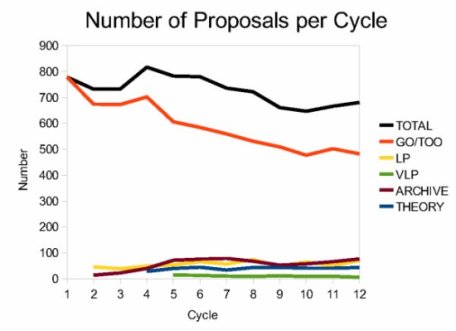
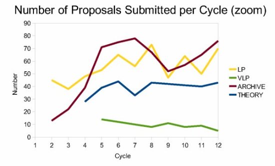
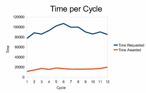
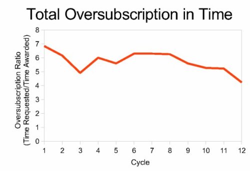
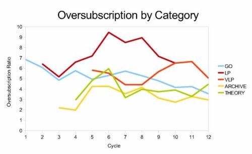
Chandra marked over eleven years of successful mission operations with continued excellent operational and scientific performance. Telescope time remained in high demand, with significant oversubscription in the Cycle 12 peer review held in June. In the Fall the observing program transitioned from Cycle 11 to Cycle 12. We released the Call for Proposals for Cycle 13 in December, and look forward to the Cycle 13 peer review in June 2011.
The team worked hard to prepare for NASA’s Senior Review of operating missions, held in April. Chandra ranked second of the eleven missions reviewed, with a score of 9.5 out of 10. In its report, the review committee observed, “After a decade in operation, Chandra remains an immensely powerful observatory in its prime, and it is well managed....Chandra has subarcsecond spatial resolution with spatially resolved spectra on the same scale. These attributes do not exist in any other mission and will not be seen again for several decades.”
The CXC conducted a workshop in February for users of the CIAO data analysis software package, a workshop in July on accretion processes, and a workshop in August on astrostatistics, as well as meetings of the Chandra Users’ Committee in April and October.
The CXC mission planning staff continued to maximize observing efficiency in spite of temperature constraints on spacecraft pointing. Competing thermal constraints continue to require some longer observations to be split into multiple short duration segments, to allow the spacecraft to cool at preferred attitudes. The total time available for observing has been increasing gradually over the past few years as Chandra’s orbit evolves and the spacecraft spends less time in Earth’s radiation belts. The overall observing efficiency during 2010 was 74%, compared with 71% in 2009. In the next several years we expect potential observing time to increase slightly, but actual observing to be limited by radiation due to increasing solar activity.
Operational highlights over the past year included seven requests to observe targets of opportunity that required the mission planning and flight teams to interrupt and revise the on-board command loads. The sun was quiet during the year, causing no observing interruptions due to solar activity. Chandra passed through the 2010 summer and winter eclipse seasons, as well as a brief lunar eclipse in February, with nominal power and thermal performance. The mission continued without a significant anomaly and with no safe mode transitions. In May the spacecraft transitioned to normal sun mode due, it is believed, to a single-event upset in an electronic circuit. The operations teams returned the spacecraft to normal status within two days with no adverse consequences and a loss of less than 40 hours of observing time.
Both focal plane instruments, the Advanced CCD Imaging Spectrometer and the High Resolution Camera, have continued to operate well and have had no significant problems. ACIS, along with the overall spacecraft, has continued to warm gradually.
All systems at the Chandra Operations Control Center continued to perform well in supporting flight operations.
Chandra data processing and distribution to observers continued smoothly, with the average time from observation to delivery of data averaging roughly 30 hours. The Chandra archive holdings grew by 1 TB to 8.3 TB and now contain 30.9 million files. 0.44 TB of the increase represents Chandra Source Catalog data products.
The Data System team released software updates to support the submission deadline for Cycle 12 observations proposals (March 2010), the Cycle 12 Peer Review (June) and the Cycle 13 Call for Proposals (December). In addition, several enhancements to instrument algorithms have been incorporated into standard data processing and also released in CIAO 4.3 (December). Chandra Source Catalog (CSC) version 1.1 was released over the summer, with the addition of the HRC imaging observations. Virtually all publicly available ACIS & HRC data for compact sources have been processed, representing on the order of 110,000 sources in the Catalog.
Education and Public Outreach (EPO) group highlights during 2010 include 11 science press releases, three press release postings, two programmatic releases, two award announcements, and 21 image releases. The group released 16 “60 second” High Definition podcasts and four longer features. The feature video “Extraordinary Universe” received the Communicator “Award of Distinction” and is a Webby Awards “Honoree.” The Mani Bhaumik award of the International Year of Astronomy (IYA) Cornerstone Project, “From Earth to the Universe” (FETTU), was presented to the Chandra EPO Principal Investigators, Kim Arcand and Megan Watzke, for the best IYA project, and the PIs were invited to give the keynote address at the IAU Communicating Astronomy Conference. Two new blog series were initiated on the CXC’s public web site, a career-focused blog, “Women in the High Energy Universe,” and a blog tracking the impact of the solar cycle on Chandra operations. Thirty-two workshops were presented at National Science Teacher Association regional and national conferences, National Science Olympiad coaches’ clinics, American Association of Physics Teachers conferences, and other state and NASA meetings.
We look forward to a new year of continued smooth operations and exciting science results. Please join us to celebrate twelve years of Chandra discoveries at special sessions of the American Astronomical Society meeting to be held in Boston in May, 2011.
Instruments: ACIS
Paul Plucinsky,
Royce Buehler, Nancy Adams-Wolk, & Gregg Germain
The ACIS instrument continued to perform well over the past year with no anomalies or unexpected degradations. The charge-transfer inefficiency (CTI) of the FI and BI CCDs is increasing at the expected rate. The CTI correction implemented in CIAO now includes a temperature-dependent component for Timed Exposure (TE) mode data and the CTI correction has been expanded to work with TE Graded mode data. See the calibration pages (http://cxc.harvard.edu/cal/Acis/detailed_info.html) and the CIAO 4.3 release notes for more details (http://cxc.harvard.edu/ciao/releasenotes/ciao_4.3_release.html). The contamination layer continues to accumulate on the ACIS optical-blocking filter. The CXC calibration group has recently released an update to the contamination model for the ACIS-I array, see the CALDB 4.4.1 release notes page for details (http://cxc.cfa.harvard.edu/caldb/downloads/Release_notes/CALDB_v4.4.1.html).
The control of the ACIS focal plane (FP) temperature continues to be a major focus of the ACIS Operations Team. As the Chandra thermal environment continues to evolve over the mission, some of the components in the Science Instrument Module (SIM) close to ACIS have been reaching higher temperatures, making it more difficult to maintain the desired operating temperature of -119.7 C at the focal plane. In previous years, a heater on the ACIS Detector Housing (DH) and a heater on the SIM were turned off to provide more margin for the ACIS FP temperature. At this point in the mission, there are two effects that produce excursions in the FP temperature, both related to the attitude of the satellite. First the Earth can be in the FOV of the ACIS radiator (which provides cooling for the FP and DH). Second, for pitch angles larger than 130 degrees, the Sun illuminates the shade for the ACIS radiator and the rear surfaces of the SIM surrounding the ACIS DH. The ACIS Ops team is working with the Chandra Flight Operations Team (FOT) to develop a model that will predict the FP temperature for a week of observations given the orientation of the satellite for each observation. Reducing the number of operational CCDs reduces the power dissipation in the FP, thereby resulting in a lower FP temperature.
Starting in Cycle 13, GOs are requested to select 5 or fewer CCDs if their science objectives can be met with 5 CCDs. GOs may still request 6 CCDs if their science objectives require 6 CCDs, but they should be aware that doing so increases the likelihood of a warm FP temperature and/or may increase the complexity of scheduling the observation. GOs should review the updated material in the Proposers’ Guide on selecting CCDs for their observations. An important point to note is that specifying “Y” for a CCD means that the CCD must be on for that observation, “N” means that the CCD must be off for that observation, and “OPT#” means that the CCD may be on for that observation if thermal conditions allow. In order to ensure that no more than 5 CCDs are used for an observation, the GO must set 5 CCDs to “N” and 5 CCDs to either “Y” or “OPT#”.
The control of the ACIS electronics temperatures has also been a concern for the ACIS Operations Team. ACIS has three main electronics boxes, the Power Supply and Mechanisms Controller (PSMC), the Digital Processing Assembly (DPA), and the Detector Electronics Assembly (DEA). The PSMC reaches its highest temperatures when the satellite is in a “forward Sun” configuration, pitch angles between 45-60 degrees (Chandra cannot point within 45 degrees of the Sun). Since 2006, the Chandra FOT has been using the optional CCDs information provided by GOs to turn off optional CCDs if thermal conditions require. As a result of the changing thermal environment, the DEA and DPA are reaching higher temperatures in tail-Sun orientations (pitch angles larger than 130 degrees). The recommendation in the previous paragraph to use only 5 CCDs if the science objectives can be met with 5 CCDs, will also reduce the temperature of the DEA and DPA in addition to the temperature of the FP. If current temperature trends continue into the future, the CXC may have to extend the turning off of optional CCDs to tail-Sun attitudes in addition to forward-Sun attitudes. GOs should always specify optional CCDs if possible to provide the maximum scheduling flexibility.
Instruments: HRC
Ralph Kraft, Mikhail Revnivstev, Mike Juda
It has been another quiet, productive year for the HRC. HRC flight operations continue smoothly with no significant anomalies or interruptions. The instrument gain continues to slowly decline with increasing charge extraction, but entirely within pre-flight expectations. We are still many years away from having to increase the operating voltage to offset the gain loss. Regular monitoring observations of Vega show no degradation in either the UVIS or the MCP photocathode. The transition of the HRC laboratory to the new space in Cambridge Discovery Park has been completed. The HRC POC is now operational again and ready to support any spacecraft/instrument anomalies.
A novel operating mode was tested
and successfully implemented in a GO observation of the Crab
Nebula over the past year. This operational mode will be
useful to anyone trying to use the HRC at its highest time
resolution on bright sources that saturate the telemetry. This
mode does not make use of the shutter. High time resolution
observations are not possible with the HRC in its default
configuration if the telemetry rate (188 cts s-1) is exceeded
because the timestamp on individual events is incorrect. In
this observation of the Crab Nebula (with LETG inserted to act
as a filter), the trigger level threshold was adjusted so that
the observed rate from the source was less than the
telemetered rate. This effectively eliminates the lowest pulse
height events from triggering the readout electronics - the
higher the threshold limit the higher the pulse height
required to trigger. Figure 8 contains a plot of both the
total and telemetered rates as a function of trigger
setting. For a trigger setting above ~ 48, both the total and
telemetered rates drop below the telemetry limit, thus
allowing timing observations at the full resolution (~ 16
μs). This mode can now be used by any GO, if desired,
to observe the small number of sources that exceed the
Chandra/HRC telemetry limit and preserve the highest temporal
resolution.
Figure 8: Total and telemetered HRC-S rates as a function of trigger threshold setting for an observation of the Crab Nebula. As the trigger setting is increased, progressively smaller pulse-height events will not trigger the event processing electronics. Once the total event rate falls below the HRC telemetry limit, full (16 μs) temporal resolution is recovered.
Figure 9: K filter image of the IGR
J17505-2644 field from UKIDSS GPS DR3 with Chandra
positional uncertainty overplotted. Magenta circle
denotes single source marginally visible inside X-ray
error box.
The HRC-I and HRC-S were used for a number of scientific investigations during the past year. We describe a study using the HRC-I to identify counterparts to Galactic low mass X-ray binaries (PI: Mikhail Revnivtsev).
Apart from being hosts for exotic objects like black holes and neutron stars, low mass X-ray binaries (LMXBs) attract a lot of attention as compact binary systems. Indeed, understanding of their secular evolution can give us insights about the rate of events extremely important in astrophysics, like: 1) SN Ia, standard cosmology candles; 2) mergers of compact objects (like white dwarf-white dwarf, neutron star-neutron star), which are crucial for our understanding of gravitational wave signals and construction of future gravitational wave detectors.
Orbital periods of LMXBs evolve very slowly, making it challenging to observe their change. However, it is clear that secular evolution of long lived LMXBs directly influences overall statistical properties of their population such as their distribution over orbital periods or X-ray luminosities. Therefore, by measuring statistical properties of galactic LMXBs, one can make important conclusions about mechanisms of their long-term evolution. The ultimate sample for this purpose is the set of persistent sources, because one can reliably estimate time averaged mass transfer rate from their instantaneous X-ray luminosity, which is impossible in case of transient objects.
In order to link the properties of binary systems with their statistical distributions, we need to measure main parameters of LMXBs, such as orbital periods, type of donor star, and others. These detailed studies are only possible for systems within our Galaxy. But even for them it has not yet been completed in a systematic manner, while considerable efforts were invested in such projects. The chance to measure LMXB orbital parameters strongly increases if the binary system harbors a giant companion because such systems are brighter in optical/IR spectral bands and they are easier to identify.
At the moment the main problem in obtaining a large complete sample of optical/IR counterparts of Galactic LMXBs is that the astrometric position of the majority of them is not known with appropriate accuracy. This is especially true for sources only recently discovered via surveys, such as the survey of the INTEGRAL observatory. A set of CHANDRA/HRC observations was requested to obtain the best possible astrometric position of X-ray sources. One of the optical fields with the HRC identified counterpart is shown in Figure 9. As a result of these observations we were able to identify IR counterparts of some of the observed sources. The remaining sources were recently covered with VVV infrared survey (VISTA Variables in The Via Lactea) and results of their identification will be published soon.
References
Zolotukhin I., 2009, ATel, 2032, “ Possible optical counterpart of IGR J17254-3257’’
Zolotukhin I.Y., Revnivtsev M. G.,2010, MNRAS, 1750 “Sample of LMXBs in the Galactic bulge - I. Optical and near-infrared constraints from the Virtual	Observatory”
Important Dates for
Chandra
Cycle 13 Proposals due: March 15, 2011
Cycle 13 Peer Review: June 20-24, 2011
Workshop: July 12 - 14, 2011
Structure in Clusters and Groups of Galaxies in the Chandra Era
CIAO Workshop: August 6, 2011
Cycle 13 Cost Proposals Due: Fall 2011
Users’ Committee Meeting: October, 2011
Einstein Fellows Symposium: Fall 2011
Cycle 13 Start: December, 2011
Cycle 14 Call for Proposals:
December, 2011
Instruments: HETG
Dan Dewey, for the HETG Team
HETG Status and Calibration
The HETG continues to perform well
with stable responses that are well
modelled by the MARX ray-trace
simulator (now at version 5.0,
http://space.mit.edu/cxc/marx/
). Activities in the past year have
enhanced the calibration for the
continuous-clocking (CC) modes with
the HETG; the results are summarized
in the POG, section 6.20.4,
“Choosing CC-Mode for
Bright Source
Observation.”
Figure 10: Comparing the Einstein/FPCS spectrum of the very bright and extended Puppis A SNR (top, from Figure 2 of Winkler et. al 1981) with the HETG/MEG spectrum of SN 1987A early in its SNR phase (bottom). This energy range includes the Ne IX He-like triplet (905–922 eV) which is somewhat resolved by the FPCS and cleanly resolved by the HETG. The SN 1987A spectrum was created online in a minute or two using TGCat, http://tgcat.mit.edu/ (Huenemoerder et al. 2011).
HETG Technique: He-like Triplets
The HETG and the XMM-Newton RGS were the stars of a high-resolution spectroscopy conference at Utrecht last year; talks and posters are online and the proceedings will be coming out soon (Kaastra & Paerels, ed.s, 2011). One of the review articles gives a thorough presentation of “He-like ions as practical astrophysical plasma diagnostics: From stellar coronae to active galactic nuclei” (Porquet, Dubau, and Grosso 2011). Our view of He-like triplets in extra-solar objects has been revolutionized by the Chandra and XMM-Newton grating instruments, though we did have a glimpse of the triplets in the days of the Einstein observatory. The focal plane crystal spectrometer (FPCS, Canizares et al. 1979) resolved Oxygen and Neon He-like triplets in some astrophysical sources, for example the Puppis A supernova, Figure 10. The complete FPCS observations and results are given in a paper by Lum et al. (1992). Since current grating spectrometer resolution is degraded for very extended sources, these data are still our highest-resolution spectrum of Puppis A!
The relative intensities of the three lines in a triplet can be described by two parameters, typically expressed by the “R” and “G” ratios reviewed in Porquet, Dubau, and Grosso 2011. Figure 11 shows examples of the HETG-observed He-like triplets of Si, Mg, Ne, and O and the corresponding parameter confidence contours in R-G space. In addition to temperature and density, the UV radiation field can also affect the triplet ratios; Mitschang et al. (2010) use this to conclude that these lines originate well within a stellar diameter of the O-star's surface.
HETG Science: Absorbing Complexities
The continuum emission from
accretion-powered sources is generated
near the compact object and has to
make its way out of the system for us
to see it. Absorption along this path,
often from ionized or 'warm'
material, can be seen in the spectra
and used to constrain the system
geometry and properties. A recent
paper by Andrade-Velázquez et
al. (2010) includes a re-analysis of
236 ks of HETG data on the Seyfert 1
galaxy, NGC 5548, located at z ~ 0.017
(~ 70 Mpc). Because of the low
foreground NH of ~ 1.6e20/cm2, the
observation provides reasonable flux
even at longer wavelengths (Figure
12). Their paper demonstrates that the
time-averaged warm absorber features
can be fit with a combination of two
outflows of distinct velocities (-490
and -1110 km/s), with each outflow
composed of two ionization
phases. This modeling is in good
agreement with velocities and
densities seen in UV spectra and may
constrain the wind geometry of the
system.
Figure 11: He-like triplets in the spectrum of θ2 Ori A, a 5th magnitude triple star system at the heart of the Orion Nebula Cluster. The data, left, are from 16 obsids totaling 520 ks of quiescent exposure. The allowed contours, right, show a strong decrease of the R ratio from high-Z (Si) to low-Z (O) elements, due to the star’s UV flux. From Mitschang et al. (2010).
Figure 12: HETG/MEG spectrum of NGC 5548 with a complicated warm absorber model in red (see text). From Figure 9 of Andrade-Velázquez et al. (2010).
A multi-observatory campaign was carried out on the black hole candidate Cygnus X-1, producing spectra over the 0.8 to 300 keV range (Nowak et al. 2011). The Chandra HETG joined RXTE and Suzaku for one epoch of observing and proved very useful by showing the spectral complexity of the absorption which the other instruments are unable to resolve. As an example, the 30 ks HETG observation was divided into 4 based on the 'dipping' state of the source and shows that the ionization state changes with the degree of dipping, Figure 13.
Not all absorption features are so
pronounced as in the previous
examples. In Figure 14 an absorption
feature is seen between the K-alpha
and K-beta fluorescence lines in a
neutron star (NS) binary, 1A
0535+262. These data were taken with
Director Time during a 2009
“Type II”
outburst. The model does require that
Fe be over-abundant and suggests an
outflow velocity of ~ 3000 km/s
(Reynolds and Miller 2010); these high
velocity winds may be unique to
neutron star binary systems. In the
near term, the three most important
tools to make further progress in this
area are: data, data, and data.
Figure 13: Far Top: Si absorption spectra at different dipping stages of Cygnus X-1, from Miskovicova et al. (2010). As the flux is reduced during dipping (from top to bottom) the absorption shows additional features from lower ionization stages, Si IX and Si X. This suggests the dipping is due to intervention of low-temperature, high-density clumps. Top: Schematic of the Cyg X-1 system. The black hole and its accretion disk are within the small black circle; the color coding indicates the density of the companion’s focused wind (low-to-high: blue-to-red). The dipping is seen when we observe through the densest part of the wind, along the black line at orbital phase ~ 0. Figure from Hanke et al. (2009).
Figure 14: HETG/HEG high-energy region of the spectrum of the Be/X-ray binary 1A 0535+262 taken near the end of its 2009 giant outburst. The observed absorption feature, labeled “Fe XXV”, is modeled using XSTAR and must consist of several Fe ions at a common outflow velocity of ~ 3000 km/s, shown inset. From Reynolds and Miller (2010).
References
Andrade-Velázquez, M., et al. (2010) ApJ 711, 888.
Canizares, C.R. et al. (1979), ApJ 234, L33.
Hanke, M. et al. (2009), a talk at “Chandra's First Decade of Discovery”, available at: http://cxc.harvard.edu/symposium_2009/proceedings/session_14.html
Heunemoerder, D.P. et al. (2011), AJ accepted
Kaastra, J. and F. Paerels (ed.s), proceedings of the “High-resolution X-ray spectroscopy: past, present, and future” conference, Utrecht, The Netherlands, March 15-17 2010, published by Space Science Reviews. See also online material at: http://www.sron.nl/xray2010/
Lum, K.S. et al. (1992), ApJSS 78, 423.
Miskovicova, I. et al. (2010) a poster at the Utrecht “High-resolution X-ray spectroscopy” meeting (see Kaastra and Paerels reference), online at: http://www.sron.nl/files/HEA/XRAY2010/posters/6/6.09_miskovicova.pdf
Mitschang, A.W. et al., (2010). ApJ submitted. arXiv:1009.1896
Nowak, M.A. et al. (2011) ApJ 728, 13.
Porquet, D., Dubau, J, and Grosso, N., (2011) to appear in Kaastra & Paerels, above. arXiv:1101.3184
Reynolds, M.T. and Miller, J.M. (2010) ApJ 723, 1799.
Winkler, P.F. et al. (1981), ApJ 246, L27.
Instruments: LETG
Jeremy J. Drake
LETGS: Carbon
Carbon. It’s everywhere these days. Popularized by the spewing chimneys of the industrial revolution and explained by Fred Hoyle's 12C resonance that facilitates Bethe's triple-alpha process in stellar nucleosynthesis. They make everything with it now: aeroplanes, racing cars, bicycles, tennis rackets, musical instruments, footprints, everything. They even use it to make optical blocking filters for X-ray satellites. But despite its moderately important role as the basis of life as we know it, carbon still has a bit of an image problem. This is perhaps partly due to it being the prime constituent of blights like soot, gunk, grime and crud, which X-ray instrument builders refer to euphemistically as “contamination”. It doesn't help that carbon also proves to be rather messy under the X-ray microscope of high-resolution spectroscopy.
Like all heavy elements, the X-ray transmittance of carbon near its ionization threshold, between about 40 and 45 Å (0.3 – 0.28 keV), shows complex X-ray absorption near-edge structure (XANES). This would be all well and good – we could use this structure as a spectroscopic tool to study carbon in the cosmos, as has been done for elements such as O, Ne and Fe (Juett et al. 2004, 2006) – were it not for our carbon filter-clad instruments showing the same structure. It’s not quite the same structure though, and this makes it all the more messy.
The optical and UV blocking filters on the Chandra detectors are made from aluminium-coated polyimide. The polyimide (C22H10N2O5) substrate in these metal-polymer foils provides the flexural and tensile strength needed for the filter to survive the rigors of launch, while the carbon also helps attenuate UV and optical light. The energies of inner-shell states in carbon whose valence electrons are bound up in a polymer such as this are perturbed relative to those in isolated carbon atoms. The detailed structure and energies of absorption resonances of a given element then depend on its ionization and chemical state. Accurate calculation of this photoabsorption cross-section for complex materials such as polyimide is currently not readily tractable and consequently the ACIS and HRC filter transmittances as a function of wavelength used to construct the Chandra effective areas are based on measurements obtained in the laboratory and at synchrotron facilities. These calibration measurements do a pretty good job of matching most of the resonance features seen near the carbon edge in LETG observations. Pretty good, because for many sources the filter signature dominates, but we would not expect a perfect match because of carbon absorption in the source, and in the intervening interstellar medium.
While detailed photoabsorption cross-sections complete with resonance structure cannot yet be readily computed for complicated chemical compounds, they can be computed for single atoms and ions. Indeed, the use of K-edge resonance structure for studying elements like O and Ne in the ISM was made possible by such computations (Garcia et al. 2005; Gorczyca 2000). Similar calculations for carbon should, at least in principle, enable the same sort of studies for C to be made. Moreover, an accurate cross-section for the cosmic absorbers should provide a check on the propriety of the instrument absorption features and calibration in the vicinity of the edge.
Such calculations were taken on by Tom Gorczyca and his graduate student, Fatih Hasoglu, at Western Michigan University (Hasoglu et al. 2010). An example of how the resulting cross-sections look is illustrated for C II in Figure 15; similar calculations were performed for C I, III and IV ions. Also shown in Figure 15 is the cross-section computed using an independent particle approach – essentially a mean-field approximation in which the detailed interactions of the 1s electron under consideration with other electrons in the ion are not taken into account. These more simplified cross-sections are characterized by ionization edges that are essentially a step-function at the ionization threshold, and are similar to those included in ISM X-ray absorption models in common use. The resolving power of the LETGS at these energies is about 1000 (0.3 eV or so) and it might be appreciated by the comparison that the resonance structure will have an impact on observations for sources in which the cosmic absorption optical depth becomes comparable to that of the filter.
Figure 15: C II photoabsorption cross-section from detailed calculations carried out by Fatih Hasoglu and coworkers, compared to the earlier simplified independent-particle approach results of Reilman & Manson (1979). From Hasoglu et al. (2010).
Figure 16: Carbon K-edge region of the X-ray spectrum of the bright blazar Mkn 421 observed by the Chandra LETG+HRC-S. The edge absorption is mostly due to the polyimide UV-optical/ion blocking filter on the HRC-S instrument, although ISM absorption contributions are also present. Two fits to a power-law continuum model with photon index Γ=2.0, absorbed by an intervening ISM corresponding to a neutral H column density of 1 × 1020 cm-2, are shown. These differ significantly only in the carbon cross sections employed: the neutral C I cross-section of Balucinska-Church & McCammon (1992); and the C I, C II, and C III cross sections containing detailed resonance structure. In the latter case, the C ion fractions were 20% C I, 60% C II, and 20% C III. The effect of the C II resonances is clearly visible in the vicinity of 43 Å. From Hasoglu et al. (2010).
We turned to our trusty blazar calibration source, Mkn 421, to test an ISM absorption model using the new high-resolution C cross-sections. This source was caught in a very high state during an LETG+HRC-S observation on 2003 July 1 and 2 (ObsID 4149; see Nicastro et al. 2005 for a full description). An absorbed power-law continuum model has never produced a really good fit to this spectrum in the vicinity of the main C resonances. Trying a fit with an ISM absorption model that included the new high-resolution C cross-sections was instead quite revealing. The fit used a power-law continuum with photon index Γ = 2 and ISM absorption corresponding to cosmic metal abundances and neutral hydrogen column density of NH = 1.5 × 1020 cm-2 – slightly different to the parameters adopted by Nicastro et al. (2005), but here we optimized the fit to the C edge region. Immediately apparent was a precise coincidence between the C II 1s2s22p2 (2P, 2D ) resonances and a discrepancy in the same fit performed using the step function edge employed in the Balucinska-Church & McCammon (1992) absorption model. The redshift of the C II absorber is zero, indicating that it resides along the line-of-sight in our Galaxy. The new C model could not help a 5% – 15% under-prediction of the data in the 42 – 44 Å range though, but since this was just an informal test and most Newsletter readers will never read this far into the article, we just cheated a bit and added a broad Gaussian-like correction to the effective area to fix it. The fraction of the ISM carbon to atribute to the different C charge states could then be computed using rigorous statistical methods. It could be, but I just did it by eye and got 20% C I, 60% C II, and for good measure, 20% C III. This fit is illustrated in Figure 16, together with one using the Balucinska-Church & McCammon (1992) step function absorption model. The new high resolution photoabsorption cross-section data for carbon are available from Tom Gorczyca on request.*
So, the improvement in the fit is perhaps not so dramatic? Keep in mind that the ISM column toward Mkn 421 is very low compared with most Galactic lines of sight that will exhibit much stronger ISM features. We still need to look in more detail at the broad Gaussian cheat in the 42 – 44 Å region to determine if it really does warrant inclusion in the instrument calibration, or if it might be explained by other means. Any calibration updates for the region close to the C edge will likely be included later in the year, together with planned revisions to the HRC-S quantum efficiency at λ > 44 Å. There is also a weak absorption feature near 42.2 Å in the observed spectrum suggestively close to the predicted C III 1s2s22p (1P ) resonance that bears further study; absence of a stronger feature tells us that at most only about 20% of the carbon in the line-of-sight is in the form of C2+: Galactic interstellar crud is not highly-charged.
References
Balucinska-Church, M., & McCammon, D. 1992, ApJ, 400, 699
Garcia, J., Mendoza, C., Bautista, M. A., Gorczyca, T. W., Kallman, T. R., & Palmeri, P. 2005, ApJS, 158, 68
Gorczyca, T. W. 2000, Phys. Rev. A, 61, 024702
Hasoglu, M. F., Abdel-Naby, S. A., Gorczyca, T. W., Drake, J. J., & McLaughlin, B. M. 2010, ApJ, 724, 1296
Juett, A. M., Schulz, N. S., & Chakrabarty, D. 2004, ApJ, 612, 308
Juett, A. M., Schulz, N. S., Chakrabarty, D., & Gorczyca, T. W. 2006, ApJ, 648, 1066
Nicastro, F., et al. 2005, ApJ, 629, 700
Reilman, R. F., & Manson, S. T. 1979, ApJS, 40, 815
*thomas.gorczyca@wmich.edu
Recent Updates to Chandra Calibration
Larry P. David
There were four updates to the Chandra calibration data base (CALDB) released during 2010. These releases contained the standard quarterly calibration of the ACIS gain and the yearly calibration of the HRC gain. Since the ACIS charge particle background varies during the solar cycle, a new set of blank field ACIS background images was released during the past year to assist observers in the analysis of extended sources. These background images were compiled from ACIS observations taken from late 2005 through 2009 (Epoch E). In addition, a blank field HRC-I background image and a HRC-I PI background spectrum were released during 2010. A recent LETG observation of the Crab nebula revealed some remaining cross-calibration issues between the transmission efficiency of the higher orders relative to the first order. The photon statistics in the Crab data were sufficient to allowed a re-calibration of the higher order transmission efficiencies, up to seventh order. Further updates to the ACIS-I molecular contamination model and a slight revision to the HRC-I QE, to improve cross-calibration with the other focal plane detectors, were also released to the public in 2010.
With CIAO 4.3 and CALDB 4.4.1 (released on Dec. 15, 2010), ACIS data telemetered in graded mode is now corrected for the effects of charge transfer inefficiency (CTI) by default. With the current versions the CALDB and CIAO, all timed event (TE) mode data, taken in either Faint (F), Very Faint (VF) or Graded (G) telemetry format is corrected for the effects of CTI by default. The calibration team is presently working on methods of applying CTI-corrections to continuous clocking (CC) mode data. Users can also apply temperature-dependent gain corrections to ACIS data with the latest versions of the CALDB and CIAO. A discussion of what data should be re-processed with the new temperature-dependent gain correction software is given at http://cxc.harvard.edu/contrib/tcticorr.
The Chandra calibration team continues to support the efforts of the International Astronomical Consortium for High Energy Calibration (IACHEC). The CXC helped organize the 5th annual IACHEC meeting which took place in April, 2010 in Woods Hole, Massachusetts. These meetings bring together calibration scientists from all present and most future X-ray and γ-ray missions. Collaborations among the calibration scientists have produced two papers that describe the present cross-calibration status between Chandra, XMM-Newton and Suzaku using clusters of galaxies (Nevalainen, David & Guainazzi 2010, A&A, 423, 22.) and the supernova remnant G21.5-09 (Tsujimoto et al. 2011, A&A, 525, 25.)
CIAO 4.3: pushing the Chandra spatial resolution to its limit
Antonella Fruscione, for the CIAO team
Version 4.3 of the Chandra Interactive Analysis of Observation (CIAO) and CALDB 4.4.1, the newest versions of the Chandra Interactive Analysis of Observations software and the Chandra Calibration Database were released in December 2010.
CIAO 4.3 includes several enhancements and bug fixes with respect to previous CIAO versions. One of the most important facilitates significant improvement to the already unprecedented spatial resolution of Chandra X-ray imaging with the Advanced CCD Imaging Spectrometer (ACIS) through subpixel event repositioning techniques.
As outlined in the CIAO “Why topic” “ACIS Sub-Pixel Event Repositioning (http://cxc.harvard.edu/ciao/why/acissubpix.html), for sources near the optical axis of the telescope, the size of the point spread function is smaller than the size of the ACIS pixels (< 0.49 arcsec). Li et al. (2003, 2004) describe various subpixel event repositioning algorithms that can be used to improve the image quality of ACIS data for such sources. Their algorithm “EDSER” (Energy-Dependent Subpixel Event Repositioning) can be applied to all Chandra observing modes - except for CC mode - and to data on both front-illuminated and back-illuminated CCDs. As of CIAO 4.3 this algorithm has been incorporated into the tool acis_process_events. It is therefore possible to reprocess older data to apply a subpixel algorithm. As of version DS 8.4 of the Standard Data Processing (SDP) code in the pipeline (planned for the spring of 2011), the default processing will also apply this subpixel algorithm. Note that most users will not notice a difference in the data with the “EDSER” subpixel resolution applied. The exception is users working with high-resolution (< 1 arcsec) data on-axis. Figures 17 and 18 show examples of optimized image resolution by subpixel repositioning of individual X-ray events.
On the “instrument
response” front, a
substantial and important improvement
has been added in CIAO 4.3 regarding
ARFs (Ancillary Response
Functions). Via the tool arfcorr it is
now possible to correct an ARF for the
finite extraction region, while
sky2det is an improved weighting
algorithm to account for spatial
variations in the ARF. arfcorr
calculates the approximate fraction of
the point spread function (PSF)
enclosed by a region, which the tool
then applies in an energy-dependent
correction to the ARF file. sky2det
creates a weighted map (WMAP) used by
mkwarf: it properly weights the ARF
based on how much of the source flux
fell onto the bad pixels, columns, or
a node boundary and which bad pixels
are actually exposed. Without
accounting for these effects, the ARF
is significantly over-estimated.
Figure 17: Three examples of optimized image resolution by subpixel repositioning of individual X-ray events. From Kastner et al (2002) (figures 3, 4 and 5 in the paper), X-ray images of planetary nebulae BD +30°3639 (panel a), NGC 7027 (panel b) and NGC 6543 (panel c). The left panels X-ray images are obtained by binning events before removing position randomization and applying subpixel event position corrections (“original” image). The center panels are images obtained by binning events after removing event position randomization (“unrandomized” image). The right panels are images obtained by binning events after removing randomization and applying subpixel event position corrections (“event relocated” image). The comparisons between “original”, “unrandomized”, and “event relocated” images illustrate the superior spatial resolution afforded by subpixel event repositioning.
A substantial effort has been invested during the past year in the CIAO contributed scripts package. This contains analysis scripts and modules written by scientists and IT specialists at the CXC to automate repetitive tasks and extend the functionality of the CIAO software package. The CIAO Scripts Package is installed seamlessly within the CIAO structure and is considered a required part of the installation; however new scripts or updates are released more often than CIAO, generally once a month.
Recent notable additions include:
chandra_repro: a reprocessing script which automates the recommended data processing steps presented in the CIAO analysis threads and may be used to reprocess ACIS and HRC imaging data.
combine_spectra: a script which sums multiple imaging source PHA spectra, and optionally, associated background PHA spectra and source and background ARF and RMF instrument responses; the script utilizes the new tool addresp which adds multiple RMFs, weighted by ARFs and exposures and adds multiple ARFs, weighted by exposures.
specextract: an improved python-version of the old tool by the same name, which now lets the user create source and background PHA or PI spectra and their associated unweighted or weighted ARF and RMF files for point and extended sources .
make_psf_asymmetry_region: a script which creates a region file indicating the location of the PSF asymmetry found in HRC and ACIS data as described in “Probing higher resolution: an asymmetry in the Chandra PSF” (http://cxc.harvard.edu/ciao/caveats/psf_artifact.html).
Forthcoming (in spring 2011) is a complete rewrite and improvement of the merge_all script to combine any number of observations and create corresponding exposure maps and exposure-corrected images.
Other notable CIAO 4.3 changes and improvements are within Sherpa, the modeling and fitting package, which now supports model expressions with different types of instruments and combinations of convolved and non-convolved model components, and caching of model parameters. It also has improved support for multi-core processing, new iterative fitting methods and many new high level user interface functions (see also the article by Siemiginowska et al. in this newsletter). The ChIPS plotting application includes support for creating axes with WCS meta data associated with them (Figure 19 ). There are new commands for panning and zooming in plots, as well as improved image support and many enhancements and bug fixes. Finally the Data Model supports tab separated values (TSV) format ASCII files, including the extended header detail provided by the Chandra Source Catalog (CSC) output format.
Users interested in hands-on CIAO training should plan to attend the next CIAO workshop which will be held in Cambridge, MA, USA on 6 August 2011 immediately following the X-Ray Astronomy School. More information will be posted at http://cxc.harvard.edu/xrayschool/ and http://cxc.harvard.edu/ciao/workshop/.
More information and updates on CIAO can always be found at: http://cxc.harvard.edu/ciao/.
To keep up-to-date with CIAO news and developments subscribe to chandra-users@head.cfa.harvard.edu (send e-mail to ‘majordomo@head.cfa.harvard.edu’, and put ‘subscribe chandra-users’ (without quotation marks) in the body of the message).
A few important notes for CIAO users:
1. Switching to Python
As of CIAO 4.3 only the Python interface is supported in CIAO. Old and new users of CIAO should learn the Python syntax for ChIPS and Sherpa. However the CXC is committed to helping existing S-Lang users transition to Python; contact Helpdesk if you need assistance.
2. SherpaCL
The sherpacl application has not been updated to work in CIAO 4.3. Please contact the Helpdesk if you would like to use SherpaCL in CIAO 4.3.
3. CIAO 3.4 and CALDB3.x
The CXC no longer supports CIAO 3.4 however the CIAO3.4 webpages will stay on-line for the foreseeable future. Similarly there will be no more updates for version 3.x of the CALDB: CALDB3.5.5 is the last CALDB updated for CIAO3.4. All the latest calibration updates are not included in CALDB 3.x. We encourage users to migrate to CIAO 4.3 and CALDB 4.4.1. We also note that CALDB 4.x is not compatible with CIAO3.4.
References
		Kastner J.H., Li J., Vrtilek S.D., Gatley I., Merrill K. M., Soker N., 2002, ApJ, 581, 1225
		Li J., Kastner J.H., Prigozhin G.Y., Schulz N.S., 2003, ApJ, 590, 586
		Li J., Kastner J.H., Prigozhin G.Y., Schulz N.S., Feigelson E.D., Getman K.V., 2004, ApJ, 610, 1204
		Wang Junfeng, Fabbiano G., Risaliti G., Elvis M., Mundell C.G., Dumas G., Schinnerer E., Zezas A., 2011, ApJ, 728, 1
Figure 18: From a paper by Junfeng Wang and collaborators (2011) a comparison between ACIS images of the inner 3"-radius circum-nuclear region in the Seyfert 1 galaxy NGC 4151 before and after subpixel repositioning. (a) Raw 0.3-1 keV ACIS image; (b) Same image after SER algorithm (Li et al. 2004) and subpixel binning (1/8 native pixel), demonstrating the improved resolution. Note the 1 arcsec scale.
Figure 19: A Chandra three-color image of the supernova remnant Cassiopeia A (Cas A) represented within a ChIPS window with RA and Dec axis. The bottom panels show three-color images of Spitzer and DSS, with the contour showing the total Chandra intensity.
Sherpa, Python and Optimization
Aneta Siemiginowska
The latest version of Sherpa was released in December 2010. Sherpa is a modern modelling and fitting Python application in CIAO, can also be run as a standalone package in a Python shell. Sherpa contains a powerful language for combining simple models into complex expressions that can be fit to the data using a variety of statistics and optimization methods. Sherpa is also easily extensible to include user models, statistics and optimization methods and methods provided by the user.
CIAO users can start Sherpa by simply typing “sherpa” on the command line within the CIAO environment. This gives access to all the Sherpa high-level user functions and also provides access to the most of the internal data and variables. Other Python packages (for example, scipy) can be imported to a Sherpa session just as in any other Python applications.
To access Sherpa from a Python shell independently of CIAO, one needs to “import sherpa”. This option is convenient for non-X-ray astronomers who would normally not work in CIAO.
The following two web pages provide more information about Sherpa for CIAO and Python users:
Sherpa Modeling and Fitting in CIAO:
http://cxc.harvard.edu/sherpa/
Sherpa Modeling and Fitting in Python:
http://cxc.harvard.edu/contrib/sherpa/
Python in Astronomy
Programming languages and programing styles evolve. Like scientific ideas, they become more and less fashionable. Only a few of the compiled languages (e.g., Fortran, C) have lasted for decades. Python is a “scripting” (not-compiled) language that has become more and more popular in the astronomy community. There are many packages for data analysis being developed in Python, e.g. PyRAF, Fermi software, CASA. Also there are many new web pages presenting Python software to astronomers (for example astropython http://www.astropython.org/ or astrobetter) and conferences devoted to scientific analysis performed in Python.
Python turns out to be an easy language to use for scientists. It is very useful in every day scientific programing. It is also relatively easy to incorporate a code written in C (or Fortran) into Python. Python's scientific libraries contain many useful functions and tools. Over the last few years Python has matured and become stable, yet it is still an active language with plenty of community support. Unlike IDL, scientific Python software is free. In addition, Linux and Mac users get a version of Python as a standard part of their operating system installation.
Sherpa development in Python started a few years ago when the language was not as popular as today. Large parts of the Sherpa code have been kept as C, but the main user interface has been developed in Python. The first Python version of Sherpa was released in December 2009. The second update was available last summer and a fully updated new version was released last December (2010).
Sherpa Capabilities
Sherpa allows users to:
Fit 1D (multiple) data including: spectra, surface brightness profiles, light curves, general ASCII arrays
Fit 2D images/surfaces in the Poisson and Gaussian regimes
Build complex model expressions
Import user-defined models
Use appropriate statistics for modelling Poisson or Gaussian data
Import user-defined statistic functions, with priors if required by analysis
Visualize a model parameter space with simulations and with 1D/2D cuts
Calculate confidence levels on the best fit model parameters
Choose a robust optimization method for the fit: Levenberg-Marquardt, Nelder-Mead Simplex or Monte Carlo/Differential Evolution.
Optimization
The main scientific goal of Sherpa modelling is finding the model parameters that best describe the observed data.
The “forward-fitting” algorithm employed by Sherpa is a standard technique used to model X-ray data. A statistic, usually an assumed weighted χ2 or Poisson likelihood (e.g. Cash), is minimized in the fitting process to obtain a set of the best model parameters. Astronomical models often have complex forms with many parameters that may be correlated (e.g., an absorbed power-law); minimization is not trivial in such a setting, as the statistical parameter space becomes multimodal, and finding the global minimum is difficult. Therefore there are several optimization algorithms in Sherpa which target a wide range of minimization problems. Two local minimization methods were implemented: (1) levmar - the Levenberg-Marquardt algorithm was obtained from the MINPACK subroutine LMDIF and modified to achieve the required robustness; and (2) simplex - the Nelder-Mead simplex method was implemented in-house, based on variations of the algorithm described in the literature (Nelder & Mead, 1965, Computer Journal, vol 7, 308-313). A global search Monte-Carlo method - moncar - has been implemented following a differential evolution algorithm presented by Storn and Price (1997) (J. Global Optimization 11, 341-359, 1997; http://www.icsi.berkeley.edu/~storn/code.html).
In summary: levmar is fast, very sensitive to initial parameters, and performs well for simple models, e.g. power-law or single-temperature models, but may fail to converge with complex models. neldermead-simplex and moncar are both very robust and converge to the global minimum in complex model cases. neldermead-simplex is more efficient than moncar, but moncar probes a larger part of the parameter space. moncar or neldermead should be used when fitting complex models with correlated parameters.
User Models and Contributed Sherpa Packages
Sherpa's Python implementation makes user contributions easy. Users can develop their specific models, functions or pipelines in Python and import them to Sherpa.
There are a few contributed packages on the Sherpa web page already. The deproject package developed by Tom Aldcroft is a CIAO Sherpa extension package to facilitate deprojection of two-dimensional annular X-ray spectra to recover the three-dimensional source properties. For typical thermal models, this would include the radial temperature and density profiles. This basic method has been used extensively for X-ray cluster analysis, and the deproject package brings this functionality to Sherpa as a Python module that is straightforward to use and understand.
Two other Python packages contributed by Tom Aldcroft are: datastack which improves the user interface in analysis of multiple data sets and cosmocalc which is an implementation of Ned Wright's cosmology calculator.
pyblocxs is a result of an on-going collaboration between the Sherpa Team and the astrostatistics group CHASC. It is an MCMC-based algorithm designed to carry out Bayesian spectral fitting of low counts data (Van Dyk et al 2001, ApJ. 548, 224). It explores the parameter space at a suspected minimum using a predefined Sherpa model. It includes a flexible definition of priors and allows for variations in the calibration information. It can be used to compute posterior predictive p-values for the likelihood ratio test (see Protassov et al. 2002, ApJ. 571, 545).
Web page for the Astrostatistics Group CHASC:
http://hea-www.harvard.edu/AstroStat/
Web page for contributed Python packages:
http://cxc.cfa.harvard.edu/sherpa/contrib.html
We also have a “Sherpa Blog”, with postings from developers and other contributors. News, hints and advice can be found there: http://pysherpa.blogspot.com/.
Figure 20: An example of parameter search in Sherpa using neldermead-simplex (left) and moncar (right) optimization methods. The temperature parameter values are shown as a function of the Cash statistics. Each point represents an iteration step in the parameter value. Both algorithms converged to the same minimum, with neldermead-simplex requiring a smaller number of iterations than moncar.
Figure 21: Parameter space probed with the MCMC sampler in pybloxcs. Right panel shows parameter values tried at each iteration.
Figure 22: Histogram distribution of a parameter returned by pyblocxs. Cumulative distribution of a parameter with the median and 90% quantiles marked by vertical lines.
Chandra Related Meetings in 2011
Check our website for details:
http://cxc.harvard.edu/
12 Years of Science with Chandra
(within the AAS meeting)
May 23-25, 2011
Boston, Massachusetts
http://cxc.harvard.edu/symposium_2011/index.html
Structure in Clusters and Groups of Galaxies in the Chandra Era
July 12-14, 2011
DoubleTree Guest Suites, Boston, MA
http://cxc.harvard.edu/cdo/xclust11/
X-ray Astronomy School
August 1-5, 2011
Cambridge, MA
http://cxc.cfa.harvard.edu/xrayschool/
CIAO Workshop
August 6, 2011
Cambridge, MA
http://cxc.harvard.edu/ciao/
Einstein Fellows Symposium
Fall 2011
http://cxc.harvard.edu/fellows/
AtomDB 2.0 released
Adam Foster, Li Ji,
Randall Smith, and Nancy Brickhouse
A new version of AtomDB (Atomic DataBase), including new APEC calculations, has been released as of January 10th 2011. This database collects atomic data relevant to modeling the emission from collisionally-ionized thermal plasmas, with a particular focus on ions and processes of interest to X-ray astronomy. The data is stored as FITS files to allow for ease of use in other analysis work. In this update, the data for almost every ion in the database has been replaced, leading to significant changes in emission spectra and line diagnostics. Two versions are available now at http://www.atomdb.org: one that can be used as a drop-in replacement in Sherpa or XSPEC, and another that contains every element with Z=1-36 but requires updates to the fitting codes before it can be used.
One of the most fundamental changes has been the upgrade to the ionization and recombination rates. The old AtomDB used rates from Mazzotta et al. (1998), which have now been replaced with the more recent compilation of Bryans et al. (2009). This has a noticeable effect on the ionization balance for some important ions, such as Fe XVII, generally shifting them to higher temperatures. This in turn has affected the resulting emissivities for many lines, in particular those of Fe L-shell ions.
Recombination rates are now divided into level-resolved rates, resulting in a modest further change to line emissivities that will nonetheless impact the emission for plasmas in non-equilibrium ionization. For this reason, the ionization and recombination rate files have been included in this release for the first time to allow full non-equilibrium ionization modeling to be performed.
In addition, the collisional excitation rates for every H- and He-like ion, and for the iron L-shell ions (Fe XVII to Fe XIV) have been upgraded to a new set of R-Matrix calculations. This provides significantly improved effective collision strengths.
As a result of all of this new data, several outstanding issues raised with the old database have been solved. The figure shows the electron temperature measured using two different line ratios using the old database – in theory, these should agree, however they consistently did not. In AtomDB 2.0, the new He-like data leads to a much better agreement between the two methods.
Future developments already underway for the next release include the incorporation of the XSTAR photoionization database into AtomDB, and inclusion of new inner-shell excitation data for Li-like ions, which will be significant for non-equilibrium ionization studies. In the meantime, work is ongoing to incorporate all of the new data into analysis tools such as Sherpa, XSPEC and ISIS. As of now, the new data are directly available for public use from the AtomDB website – www.atomdb.org.
News from the Chandra Data Archive
(CDA): NEW Footprint Service
Aaron Watry, Arnold Rots
The CDA started the new year bringing online a new interface: the Chandra Footprint Service. This service provides a visual web interface to all public Chandra observations, as well as to the coverage of the Chandra Source Catalog (CSC); see Figure 24. It superimposes the instrumental coverage of the Chandra instruments on a cut-out image from the Digital Sky Survey, using the look and feel of the footprint service of the Hubble Legacy Archive (HLA).
The service provides the user with three functional tabs (in addition to Help and FAQ):
1. The main Footprint tab displays the footprint and an accompanying table of all the observations displayed in the footprint. The table is user-configurable, may be filtered, and selections are mirrored in the footprint overlay. In addition, the user can turn instruments on and off and choose between archived data (up to Level 2) and the CSC.
2. The Image Inventory tab provides a list of all the Chandra images that are available from the observations in the table.
3. The Image Preview/Data Download tab allows the user to browse those Chandra images and select observations for download through WebChaSeR.
The Footprint service is VO-compliant and can provide VOTable output.
In the future we hope to provide options to add CSC positions to the footprints and to include footprints from different missions and archives.
Figure 23: Comparison of the electron temperature implied by two different line ratio diagnostics for O VII and O VIII, using HETG observations and the old database (based on Testa+2004). The new data (shown in red for one point) significantly changes the G-ratios, correcting the discrepancy.
Figure 24: Chandra coverage around M 82. The footprint outline of ACIS-I observations is overlaid in blue, ACIS-S in red, HRC-I in green, and HRC-S in magenta. Selecting a particular observation turns its outline yellow and will highlight the corresponding line in the table (not shown).
Recent Chandra Dataset Identifiers
Sherry Winkelman, for the Archive Operations Team
Publications managed by the AAS provide authors with a mechanism that allows them to follow links in either direction between journal articles and the observational data presented therein. Identifiers are described at: http//cxc.harvard.edu/cda/datasetid.html.
The Chandra Data Archive (CDA) would like to thank our recent dataset identifier contributors. Your use of dataset identifiers greatly improves our ability to link data to published results. We have two defined sets in the past year:
1. ADS/Sa.CXO#DefSet/CCCP - contains 38 obsids related to the Chandra Carina Complex Project (http://cxc.harvard.edu/cda/DefSet/CCCP.html)
2. ADS/Sa.CXO#DefSet/GBS - contains 195 obsids related to the Galactic Bulge Survey
(http://cxc.harvard.edu/cda/DefSet/GBS.html)
We also created contributed sets for both Chandra Deep Fields which are pre-packaged datasets of the Deep Fields. They can be found at:
ADS/Sa.CXO#Contrib/2010/CDFN
(http://cxc.harvard.edu/cda/Contrib/2010/CDFN)
ADS/Sa.CXO#Contrib/2010/CDFS
(http://cxc.harvard.edu/cda/Contrib/2010/CDFS)
In addition, we are now working with the Chandra EPO group to create dataset identifiers for press releases. The first identifier is linked to the M82 press release which was issued at the January AAS and can be found at:
Dataset identifiers provide a means of linking articles and the observational data that are presented in them. Such linking provides a powerful data mining tool which the CDA uses to create its bibliography. (For more details see Chandra Newsletter #17.) In addition the ADS, CDA, and other observatories are collaborating to create a richer, semantically linked research environment by sharing information about observations and bibliographic content. Clearly labeling data in papers and using dataset identifiers play a key role in that linking.
The CDA recognizes five types of datasest identifiers to link to published Chandra results:
1. to individual observations:
ADS/Sa.CXO#obs
2. to lists of multiple observations:
ADS/Sa.CXO#DefSet
3. to static contributed data products:
ADS/Sa.CXO#Contrib/YYYY
4. to dynamic contributed data products:
ADS/Sa.CXO#Contrib
5. to the Chandra Source Catalog:
ADS/Sa.CXO#CSC
We encourage authors to use dataset identifiers in their manuscripts as a means of creating direct links to the data used in their publications. You can find details on using and requesting identifiers at the CDA website, http://cxc.harvard.edu/cda/datasetid.html.
Retirement of
Longtime Newsletter Editor: Dr. Nancy Evans
May 2010 marked the retirement of Chandra Director's Office scientist and longtime Newsletter editor, Dr. Nancy Remage Evans.
Nancy masterminded planning, designing and editing this annual, Chandra Newsletter from Issue #4 in Sep. 1996 to #17 in Spring 2010, 14 Issues in all. During this time she also oversaw several updates in format, taking advantage of newly available software to keep the Newsletter current and looking sharp and professional, both electronically and in hardcopy.
Nancy set a high standard. She diligently researched and sought out articles on all aspects of the observatory, including recent events affecting the observatory or its users, current science reviews and press releases, upcoming events, relatively routine status reports, and future mission news. The result was a consistently reliable, useful and attractive document which allowed interested readers worldwide to keep in touch with Chandra and its exciting science.
We thank Nancy for her hard work over so many years and wish her many years of happy retirement. We miss her presence in the CXC, but we enjoy the continued pleasure of her company as she continues her scientific research on Cepheid stars here at the CfA.
Reflections from the Outgoing Editor
Nancy Remage Evans
After more than a decade of editing the Chandra Newsletter (since Issue 4 in 1996, back when it was the AXAF Newsletter), I was asked by Paul Green, the new editor, if I had any thoughts to pass along. After a little reflection, I decided that my thoughts were a list of thanks for the effort from so many people which went into our annual summary.
Thanks to:
Of course the major thanks are to the team who put Chandra together and pulled it off. The “Ten Years of Chandra Conference” brought a lot of them together (2010, PNAS, 107, 2127; http://cxc.harvard.edu/ChandraDecade/). Take a look at the back page of Issue 17. The launch issue (Issue 7, 2000) celebrated with a splurge of color in the center spread. Times have changed–and we are now all color.
The hardworking science staff continuously push the science and calibration data to get the most out of it. Sometimes it takes a nudge to get them to write things up, but happily Users' Committee reports could frequently be repurposed for the whole community to use.
The writers of the “commissioned cover stories” always did a great job.
Particular thanks to Diana Worrall for starting the Newsletter and with it, the first Chandra/AXAF User database. Off to a good start.
A lot of Director's Office support staff helped with the production, with special thanks to Mihoko Yukita and Tara Gokas for moving the production into sophisticated desktop publishing–and into full color.
The article I have personally used the most was the one by Jiahong Juda on the calibration facility, and I always looked forward to anything by Wallace and Karen Tucker.
And, of course, I learned more about copyright than I ever intended. Thanks all.
And happy editing, Paul!
Figure 25: Nancy Remage Evans peruses the 2010 Newsletter (photo courtesy Jonathan McDowell).
Chandra: Promises Made and Kept
Wallace Tucker
A promise made is a debt unpaid. ~Robert Service
Chance favors the prepared mind. ~Louis Pasteur
Not long ago a request came down from above for a list of Chandra's achievements that have completely transformed the way we have viewed our world, solar system, sun, or universe.
In other words, how many discoveries of the century have you made this year?
In a bow to David Letterman, or the decimal system, or other lists of ten that you can easily summon up, Chandra Project Scientist Martin Weisskopf submitted a list of Chandra’s top ten which would probably fall beyond the event horizon, never to be seen again. Not really, because it appears below, and being an environmentally conscious group, we will likely recycle the list several times before the next request requires generation of a new list which will be similar, but not identical to previous lists because real progress is being made.
Chandra's Top Ten
(As of January 2011, not necessarily in order of importance)
1. Deep field observations resolved the X-ray background and showed that it is dominated by accreting supermassive black holes including a large number of highly obscured black holes.
2. Images of clusters of galaxies established that energetic feedback by rotating supermassive black holes dramatically affects the evolution of intracluster gas and galaxies.
3. X-ray rings and jets around rotating neutron stars provide the most direct evidence of the transformation of rotational energy of these stars into jets and winds of high energy particles.
4. X-ray and optical observations of the Bullet cluster of galaxies show the separation of dark and ordinary matter in a collision between galaxy clusters.
5. Observations of the rate at which massive galaxy clusters grow have provided confirmation that the expansion of the universe is accelerating, an effect attributed to the prevalence of dark energy, and have ruled out some alternatives to General Relativity.
6. Observations of supernova remnants showed that supernova explosions are asymmetric and turbulent, requiring mixing of layers either during or prior to the explosions, and images of supernova shock waves provide evidence for acceleration of electrons to extremely high energies.
7. Detection of absorption by highly ionized oxygen atoms in X-ray spectra of a quasar behind the Sculptor wall of galaxies provided evidence for the Warm Hot Interstellar Medium, thought to contain the missing baryons in the local universe.
8. Chandra observations of spectrally soft X-ray sources in early-type galaxies led to the conclusion that mergers, rather than accretion-driven explosions, are responsible for the Type Ia supernovas in these galaxies.
9. A number of multi wavelength studies of star clusters have provided an unprecedented look at the co-evolution of young stars and their disks in a wide variety of conditions.
10. Chandra was used to discover and/or contribute to an understanding of the X-ray emission processes from comets, the moons of Jupiter, the Io plasma torus, and the atmospheres of Venus and Mars.
The list, which could have easily been expanded to fifteen or more by including insight into the nature of stellar black holes (event horizon, rotation rate), the accretion process near black holes, the studies of the Galactic center region, starburst galaxies, etc., got me to wondering how well the promise of Chandra has been met, and whether we can possibly guess what the future holds. This led me to my personal archive to dig out copies of old proposals. The oldest was the proposal for a Large Orbiting X-ray Telescope, which was submitted to NASA in May of 1970.
The LOXT was to have two telescopes, one designed for high resolution with the capabilities approximately that of Chandra, and the other for maximum efficiency with approximately the capabilities of XMM-Newton. What did we expect to be the major accomplishments of LOXT? The following list is in order of appearance in the proposal.
L1. Detect line emission from Sco X-1 as a test to the binary star model for X-ray stars.
L2. Determine the nature of strong, transient X-ray stars.
L3. Resolve the X-ray emission from and around the Crab pulsar & detect and search for other rotation powered X-ray emitting pulsars in supernova remnants.
L4. Study the dynamics of supernova shock waves and measure the abundances of the elements in supernova remnants.
L5. Detect X-rays from supernovas in their first month.
L6. Detect X-rays from stellar coronas, stellar winds and flare stars.
L7. Determine the populations of X-ray sources for different galaxy types & their association with galactic features such as spiral arms.
L8. Resolve the X-ray emission around M87, especially the optical jet.
L9. Detect and study X-ray emission from Seyfert galaxies and QSO’s.
L10. Measure the granularity of the x-ray background.
L11. Look for shadows cast by cool intergalactic matter.
L12. Search for the missing mass in the form of ionized gas in clusters of galaxies.
L13. Set limits on the mass density of the intergalactic medium through observations of the soft X-ray background.
Given that this proposal was submitted before the launch of UHURU, when the total useful time from all the rocket flights was about 300 ksec, and the evidence for black holes, or the binary nature of compact X-ray sources, or the existence of the hot intracluster medium was still in the future, the overlap between this list and the latest Chandra list is remarkable. It is also noteworthy that Chandra has made significant advances on every one of the topics.
LOXT never made it through the budget gauntlet, but, largely because of the success of UHURU, the Einstein X-ray Observatory, a smaller version of the LOXT did survive, and the X-ray images made with its mirrors made the case for the Advanced X-ray Astrophysics Facility (AXAF), or Chandra. Perusing the various brochures being circulated in the halls of NASA and Congress in the mid-1980's, I came up the following list of prime scientific objectives:
A1. Understanding the magnetic dynamos in stars
A2. Probe the nature of the supernova process through observations of SNRs.
A3. Determine the size and thermal conductivity of neutron stars, and constrain the equation of state for matter at extreme densities.
A4. Confirm the existence of black holes on a stellar and galactic scale.
A5. Measure the distribution of dark matter on various size scales.
A6. Study the formation and the evolution of quasars
A7. Establish the contribution of various classes of discrete sources to the X-ray background
A8. Use the Sunyaev-Zeldovich effect to measure the Hubble constant.
A9. Measure the evolution of the heavy element content of the universe through observations of clusters of galaxies.
A10. Study plasma physics and particle acceleration processes in stellar coronas, supernova remnants and cosmic jets.
A11. Study the relation of high energy jets to apparently unrelated lower energy thermal phenomena such as star formation.
A12. Potential use of a growing archive of thousands of serendipitous sources to discover new types of objects, ranging from brown dwarfs to quark stars to new types of galaxies to cosmic strings.
The list contained most of the elements of the LOXT list, but the impact of the discoveries made by the Uhuru, Einstein, HEAO -A and other observatories, as well as the growing connections with other fields of astronomy and the physics of elementary particles, is evident. Black holes are now on the list and it has been established that dark matter cannot be in the form of hot gas.
A list prepared just before launch for PR purposes was similar, but shorter and less technical, and included the use of clusters of galaxies to test cosmological models.
Comparing the list of actual Chandra accomplishments with what was promised shows that Chandra has more than fulfilled the promises made. The list also shows that most of the discoveries, except the evidence bearing on double-degenerate precursors to Type Ia white dwarf explosions, were anticipated in a general way. The potential for discoveries in the solar system were mentioned in the LOXT and AXAF documents, but weren’t given much ink. The discovery of dark energy wasn’t anticipated, but it was well understood that the rate of formation of galaxy clusters would provide an important cosmological probe. I think it is also true that in every case the reality exceeded the anticipation – see the images of the Crab Nebula and the Perseus Cluster as prime examples.
It seems that astrophysical theorists deserve some credit for the close correspondence between what was promised and what was delivered. Maybe not so much for being visionary, but for their ingenuity in being able to adapt existing models and theories to the changing landscape revealed by observation.
That is not to say that there won’t be any surprises in the future with 95% of the energy density being in either in dark energy or dark matter, we are still very much in the dark! But the increasingly rapid and positive feedback between observational discoveries and theoretical modeling should give us a feeling of what to expect from Chandra in the next decade, and prepare the way for an ingenious use of the broad and deep data base that will be complemented by increasing multiwavelength coverage of the areas observed by Chandra.
There is great joy in serendipitous discoveries, and they make for good stories, but most of them are not totally unexpected - again dark energy is a notable exception, but even there, the researchers were confident they would find something of cosmic significance. Most discoveries occur because chance does indeed favor the prepared mind.
So Chandra seems well-prepared to make a wealth of discoveries in the coming years. I would give you my list, but I have already exceeded my allotment of words.
Figure 26: A schematic representation of the LOXT.
Figure 27: An illustration of Chandra.
Upbeat on Chandra's Longevity
Paul Viens and Sabina Bucher Hurley
After eleven-and-a-half years on-orbit, the Chandra X-Ray Observatory continues to provide ground-breaking science returns to the astrophysical community. When discussing Chandra in venues ranging from program reviews to conferences to lunch-time meetings with colleagues and friends, there is one question that inevitably comes to mind: “how long will it last?”. The response to this question, like a great many others, is “it depends”. It depends on many factors, many of which are out of our control. However, there is much optimism among the science and operations groups affiliated with Chandra that it will be around for a long time to come.
The overall health of the Chandra vehicle remains outstanding. The observatory has exhibited very few anomalies in its eleven-and-a-half years of operation. All subsystems are currently operating on their primary side equipment with only two exceptions, the Inertial Reference Units (IRUs) and the Mechanism Controller Electronics (MCEs). In both cases, the units were swapped to their redundant side for operational considerations and not due to unit failures. Vehicle performance has been exceptional with all subsystems meeting, or exceeding their original design requirements. There is considerable margin in most of the vehicle’s prime systems. Currently, there are no vehicle concerns that would preclude continued extensions of the mission.
The Chandra X-Ray Observatory is composed of three main elements: the Spacecraft system, the Telescope system, and the Integrated Science Instrument Module (ISIM). The figure below shows the current state of health of the major subsystem components within each of these elements. The Integrated Electron Proton Helium Instrument (IEPHIN) used as a radiation detector is the only subsystem with issues impacting performance; however, the MCP event rate data and the anticoincidence shield rate data from the High Resolution Camera provide alternative sources of radiation data to back up the IEPHIN unit.
To date, Chandra has only experienced five anomalies that impacted observations. All have been either fully resolved or are being effectively mitigated. Two of the issues are related to a faster than anticipated degradation of the vehicle’s Multi-Layer Insulation (MLI) outer layer of silverized Teflon. The degradation has caused higher than expected temperatures on the sun-facing side of the Observatory. The exact cause of this accelerated degradation is not entirely understood; however, it has been well characterized and the effects are manageable while maintaining a full and efficient observing program. Although each anomaly or technical issue has had some operational impact, all have been efficiently managed such that the effect on science was minimized or, in some cases, completely avoided. The flight and science teams quickly identified and reacted to these events, and to several anomalies with no significant impact, and are well poised to do so again for future anomalies.
Subsystem performance and the observatory’s operating environment are assessed on daily, weekly, monthly, and biannual bases to quickly identify and respond to adverse trends. To continue operating at peak performance, the Chandra spacecraft requires a set of routine maintenance activities to ensure desired performance levels. These include ephemeris updates, star camera dark current calibrations, IRU calibrations, and periodic flight software modifications. Effects of orbit evolution are also well understood and are being addressed.
In addition to the research of possible future anomalies and preparing for their occurrence, the flight team has performed considerable analysis of the probability of extending vehicle life. Analyses associated with extending vehicle life include periodic studies of life limiting factors, which analyze all mission consumables and life-limited items. These investigations have looked at lifetime projections for static hardware items such as the Multi-Layer Insulation, propulsion thrusters, heaters, and OBC flight software memory, as well as lifetime projections for dynamic hardware items such as propulsion fuel, IRU spin bearings, battery charge/discharge cycles and mechanism moves. To date, these analyses have been able to show that, given no unexpected anomalies or other mission impacting problems, there were no concerns with reaching and/or exceeding the studies’ target mission durations.
With regard to on-board consumables, of primary interest are the amount of fuel remaining for the MUPS thrusters, and budgeted allocations for items such as thruster warm starts and mechanism moves. At this point in the mission, less than 18% of the fuel in the MUPS tank has been consumed, thanks to judicious mission planning practices in managing momentum accumulation. Based on the recent fuel usage rate, there is an estimated 22 years remaining before a switch to the backup fuel supply in the IPS tank will be needed. The number of “warm starts” is also monitored closely, since a swap to the MUPS B-side will be needed if a pre-defined threshold based on qualification life testing is ever reached. A “warm start” is a thruster firing at a catalyst bed temperature of about 450 deg F, which occurs at the start of a momentum unload. The latest trends in the accumulation of warm starts suggest a swap will not need to be considered before year 19 or 20 of the mission, at which point the fresh B-side thrusters can be brought into service. The bottom line: the Chandra consumables are in good shape!
Electrical power is the life-blood of the observatory, and aboard Chandra there is plenty of power for the extended mission. All three batteries are healthy, with capacity to spare for handling future eclipse events. The solar array continues to support all of Chandra's power demand, as well as the batteries' charge needs. The degradation of the solar array’s performance is closely following the pre-launch expectations. This, along with decreasing power needs as the spacecraft heating trend continues and the on-board heaters turn on less often, suggests that long-term solar array capability will remain well above the projected spacecraft and science instrument power needs for a 20+ year mission.
Overall, Chandra vehicle health remains excellent. Although minor issues have surfaced, the operations team has ensured that these issues are non-impacting and do not threaten an extended Chandra mission. Continued diligence is being applied to subsystem performance trending and monitoring, as well as to managing thermal challenges and preparing for anomalies. At this time there are no known limitations due to degradation, consumables, aging, or obsolescence that would prevent Chandra from meeting Level 1 requirements over the course of a 20-year mission.
Figure 28: Chandra Major Subsystem State of Health
International X-ray Observatory Update
Michael Garcia
The Astro2010/Decadal report ‘New Worlds, New Horizons’ (NWNH) was released last summer, and specifically recognizes "IXO’s high scientific importance," stating that IXO is "central to many of the science questions identified by this survey." NWNH recommends IXO for robust technology development funding this decade and states that NASA should "determine an appropriate path forward to realize IXO as soon as possible" if IXO is selected by ESA as the first L-class mission. Because IXO is a joint ESA/NASA/JAXA mission it must be selected by all three agencies in order to move forward. The ESA selection process is known as ‘Cosmic Visions 2015-2025’ and should be complete by June 2011. Both large (L-class) and medium (M-class) missions are being selected.
As part of the ESA selection process, the ESA/NASA/JAXA IXO-Study team has compiled the ‘Yellow Book’, which describes both the science and technologies of IXO. The Yellow Book and supporting documents represent the end result of a thorough assessment of IXO carried out by ESA, including an assessment of the cost and technology risks of the mission. The team made a science presentation along with the other candidate L-class missions (EJSM/Laplace and LISA) in early Feb 2011.
We hope you were able to stop by the IXO booth at the recent AAS in Seattle, and pick up a flyer announcing the next IXO Science team meeting which was in Rome this mid-March. Proceedings should soon be available on the conference web site at http://www.iasf-roma.inaf.it/IXO/. If you are able to attend the May 2011 AAS in Boston, please stop by and speak with us at the IXO booth.
Significant progress has been made with both the X-ray Microcalorimeter Spectrometer (XMS) and the mirrors, the enabling technologies identified by the IXO team to the Decadal. The XMS team has fabricated and tested some of the first 4-pixel ‘hydra’ devices that would populate the outer 2 arcmin to 5 arcmin of the XMS array. These devices use one thermister to read out 4 X-ray absorbers, and have been built to the size required for IXO. These first devices are within a factor of two of the required energy resolution, and changes to the manufacturing procedure have been identified that should yield the required resolution.
The mirror teams also continue to make progress on both the silicon pore optics (SPO) in Europe and the segmented glass optics (SGO) in the US. Since last newsletter the SPO team has now measured 7.5 arcsec HPD (two reflections) at 3 keV in an x-ray test of a mirror sub-assembly. This compares to 9 arcsec a year ago. SGO sub-assemblies with 4.5" HPD (two reflection equivalent) figure have recently been made, breaking the 5" HPD barrier. When these sub-assemblies are aligned, transferred, and permanently bonded into a larger mirror sub-assembly, x-ray images as good as 9.7" HPD at 4.5 keV were obtained.
Figure 29: Improvement in HPD vs. time for silicon pore optics ‘X-ray Optics Units’ XOU-1 through XOU-7. Key upgrades to the ‘stacking robot’ which assembles the individual plates in stacks of reflecting pairs are shown. The next upgrade will include moving to a true Wolter geometry from the current conic approximation. Continued development should allow the required HPD to be achieved by late 2012.
Figure 30: Similarly, for the Segmented Glass Optics. The measurements have been done with optical metrology rather than x-ray testing and do not include the effects of mounting the individual shells in a flight like housing. As with the Silicon optics, continued development should allow the requirement to be met by late 2012.
The Aesthetics of (X-ray) Astronomy
Kim Kowal Arcand
Images capture the public’s attention. All aspects of the Chandra X-ray Observatory’s Education and Public Outreach (EPO) program integrate images – from press activities to formal classroom education. Beyond “being pretty,” images can be a vehicle that entices non-experts into learning more about the underlying science. Chandra’s unprecedented angular resolution provides X-ray images especially well-suited to communicating high-energy astrophysics results. To take advantage of this, the EPO has developed and honed innovative techniques for processing images as the mission, and imaging software, has progressed.
Each Chandra image created for the public necessarily represents a variety of decisions from the individual or team that assembled it. These choices include cropping, colorizing, smoothing, removing artifacts, and more. But how effective are these choices in both engaging the public’s interest and communicating scientific information to them?
Members of the Chandra EPO group, along with astrophysicists from the Smithsonian Astrophysical Observatory, and psychologists from the University of Otago, New Zealand, launched the Aesthetics & Astronomy (A&A) research project in 2008 to examine this issue. The first study, conducted with an online survey (see Figure 31) and in-person focus groups, included images from Chandra – such as the Whirlpool Galaxy and G292.0+1.8 - as well as from other telescopes across the electromagnetic spectrum, and probed the effects of the scientific and artistic choices in processing astronomical data.
The full results of the 2008 study are detailed in the Journal of Science Communication (and at http://arxiv.org/pdf/1009.0772) that includes the methodology, data limitations, and descriptive statistics of the study. Critical findings from the study include the need for strong narrative and textual context when presenting science images, for explicit discussion of the colors and what they represent in science images, and for a clear sense of physical scale that is helpful for comprehension, across all levels of expertise. These findings have been applied to recent Chandra print products and digital materials to help maximize the impact and learning opportunities for our audiences, and to ensure quality of material.
Building on the information we gleaned from the first study, we were awarded funds from the Smithsonian Scholarly Studies program to ask viewers to evaluate astronomical images and their corresponding descriptions across different media platforms: web, mobile, traditional print, and large format print. We expect to have some preliminary analysis of the new data in the next few months, and are already planning subsequent studies that would include eye movement tracking.
It is the goal of the A&A project to discover the most effective ways of communicating exciting discoveries through the aesthetic appeal that astronomical images can offer. With so much data and so many tools at astronomy’s disposal, are the best possible practices being employed? A&A studies can help to optimize the public representation of sometimes complex scientific information.
Figure 31: 2008 online study (astroart.cfa.harvard.edu)
Women in the High-Energy Universe
Kim Kowal Arcand
Figure 32: Women in the High-Energy Universe entry in the Chandra blog
The Chandra blog has a feature called “Women in the High-Energy Universe” at http://chandra.si.edu/blog//taxonomy/term/19. The goal is to highlight and promote the many important ways that women contribute to the pursuit of understanding the Universe through high-energy astrophysics. We've asked various women to tell us – in their own words – about their experiences and perspectives of their careers. We invite you to contact us if you would like to be included in the blog. Please email Kim Arcand (kkowal@cfa.harvard.edu) or Megan Watzke (mwatzke@cfa.harvard.edu).
Science for Chandra's Second Decade
Belinda Wilkes
As we move into Chandra's second decade of operation, with full expectation of continuation for 10 more years, we recognize that there are major science questions which Chandra has yet to address. A significant (if not driving) factor for this state of affairs is the large amount of observing time which major projects require. Fortuitously, the evolution of Chandra's elliptical, high-earth orbit over time brings us to a point where increased viewing efficiency is possible for a few years due to the lower fraction of time spent within the radiation belts.
In consultation with MSFC Project Science and the Chandra Users' Committee, the CXC announced a new opportunity for major projects to be proposed and considered through the regular cycle peer review process. The Chandra Cycle 13 Call for Proposals invites proposals for “X-ray Visionary Projects (XVPs)”, for 1-6 Msec of observing time, allowing the community to harness Chandra's powerful capabilities to address major scientific questions.
An XVP proposal should describe a major, coherent science program to address key, high-impact, scientific question(s) in current astrophysics. We envision that XVPs will result in data sets of lasting value to the astronomical community. Observational data associated with XVPs will be publicly released immediately and the delivery of data products and software by the XVP teams will be encouraged and facilitated by the CXC.
We expect 6-8 Msecs of observing time to be dedicated to XVP proposals in Cycle 13, allowing approval of one or more proposals. Due to the increased viewing efficiency, the time allocation for XVPs in Cycle 13 does not impact observing time available for GO or Large Programs. Observations associated with XVPs will be carried out during the ~1 year duration of Cycle 13, subject to scheduling constraints, except in cases where the science to be addressed requires distribution over multiple (up to 3) cycles.
We expect one or more future solicitations for XVPs in upcoming, not necessarily contiguous, cycles depending on assessment of potential science impact and available observing time, and in consultation with Chandra Project Science at MSFC and the Chandra Users’ Committee.
Cycle 13 XVP proposals will be reviewed at the regular peer review in June 2011 by the topical panels and by an XVP panel. The assessments of both will be passed on to the Big Project Panel, which includes representatives from all other panels, and will make the final recommendations for time allocation for both XVPs and LPs.
We are excited about this new opportunity which we anticipate will engage the creative and inventive energies of the community and will facilitate major new science breakthroughs with Chandra in the years ahead.
The Results of the Cycle 12 Peer Review
Belinda Wilkes
The observations approved for Chandra's 12th observing cycle are now in full swing and the Cycle 13 Call for Proposals was released on 15 December 2010. Cycle 11 observations are close to completion.
The Cycle 12 observing and research program was selected as usual, following the recommendations of the peer review panels. The peer review was held 22–25 June 2010 at the Hilton Boston Logan Airport. More than 100 reviewers from all over the world attended the review, sitting on 15 panels to discuss 681 submitted proposals (Figure 33). The Target Lists and Schedules area of our website provides lists of the various types of approved programs, including abstracts. The Cycle 12 peer review panel organization is shown in Table 1.
Table 1: Panel Organization
Topical Panels
Galactic
Panels 1, 2
Panels 3, 4
Panels 5,6,7
Normal Stars, WD, Planetary Systems and Misc
SN, SNR + Isolated NS
WD Binaries + CVs, BH and NS Binaries, Galaxies: Populations
Extragalactic
Panels 8,9,10
Panels 11,12,13
Galaxies: Diffuse Emission, Clusters of Galaxies
AGN, Extragalactic Surveys
Big Project Panel
LP and VLP Proposals
CDFS Merging Panel
CDFS archival proposals
A detailed investigation of
accepted and available observing time
was carried out in April-May 2010. Due
to a number of factors, there was
insufficient allocated observing time
in the Observation catalog to maintain
an efficient schedule throughout Cycle
11. These factors include a previously
unaccounted increase in observing
efficiency, due to the lower fraction
of time spent within the radiation
belts as Chandra’s orbit
evolves, as well as the accumulation
of unused time on TOOs. To compensate
for the resulting lack of available
targets in Cycle 11 and to correctly
account the time available in Cycle
12, the amount of time allocated at
the Cycle 12 peer review was
increased. The final time allocation
was 16% higher than in Cycle 11 at
20.08 Msecs (including TOO
probability). This is reflected in the
2010 numbers in Figure 34, which shows
the time allocated in comparison with
the time requested as a function of
cycle. Due to the larger amount of
time allocated, the final
over-subscription rate in terms of
observing time for Cycle 12 was 4.2,
significantly lower than the ~5.5 of
previous cycles (Figure 35). The total
time request was 88 Msecs, very
similar to past cycles (Figure
34).
Figure 33: (left) The number of proposals submitted in each proposal type (e.g. GO, LP, Archive etc.) as a function of cycle. (right) Zoom on lower curves. Since more proposal types have become available in each cycle, the number classified as GO has decreased as other types increase. The total number of submitted proposals is remarkably constant.
Figure 34: The requested and approved time as a function of cycle in ksecs. This increased in the first few cycles with a peak in Cycle 5 due to the introduction of VLPs. In the past few cycles it has been relatively constant. The increase in awarded time in Cycle 12 is clear in the red curve.
As is our standard procedure, all proposals were reviewed and graded by the topical panels, based primarily upon their scientific merit, across all proposal types. The topical panels produced a rank-ordered list along with detailed recommendations for individual proposals where relevant. A report was drafted for each proposal by one/two members of a panel and reviewed by the Deputy panel chair before being delivered to the CXC. The topical panels were allotted Chandra time to cover the allocation of time for GO observing proposals based upon the demand for time in that panel. Other allocations made to each panel were: joint time, TOOs with a < 30 day response, time-constrained observations in each of 3 classes and money to fund archive and theory proposals. Many of these allocations are affected by small number statistics in individual panels so allocations were based on the full peer review over-subscription ratio. Panel allocations were modified, either in real time during the review or after its completion, transferring unused allocations between panels as needed.
Figure 35: The final over-subscription in observing time based on requested and allocated time in each cycle. Again the numbers are remarkably constant until Cycle 12 where the lower value reflects the 16% larger amount of time awarded (see also Figure 2).
Large (LP) and Very Large Projects (VLP) were discussed by the topical panels and ranked along with the other proposals. The topical panels' recommendations were recorded and passed to the Big Project Panel (BPP). The BPP discussed the LPs and VLPs and generated a rank-ordered list. BPP panelists updated review reports, as needed, both at the review and remotely over the following 2 weeks. The schedule for the BPP included time for reading and for meeting with appropriate panel members to allow coordination for each subject area. The BPP meeting extended into Friday morning to allow for additional discussion and a consensus on the final rank-ordered list to be reached.
The resulting observing and research program for Cycle 12 was posted on the CXC website on 14 July 2010, following detailed checks by CXC staff and approval by the Selection Official (CXC Director). All peer review reports were reviewed by CXC staff for clarity and consistency with the recommended target list. Formal letters informing the PIs of the results, including budget information (when appropriate) and providing a report from the peer review were e-mailed to each PI in August.
Joint Time Allocation
Chandra time was also allocated to several joint programs by the proposal review processes of XMM-Newton (3 proposals) and HST (2 proposals).
The Chandra review accepted joint proposals with time allocated on: Hubble (19), XMM-Newton (1), Spitzer (1), NRAO (11), and NOAO (3).
Constrained Observations
As observers are aware, the biggest challenge to efficient scheduling of Chandra observations is in regulating the temperature of the various satellite components (see POG Section 3.3.3). In Cycle 9 we instituted a classification scheme for constrained observations which accounts for the difficulty of scheduling a given observation (CfP Section 5.2.8). Each constraint class was allocated an annual quota based on our experience in previous cycles. The same classification scheme was used in Cycles 10-12. There was a large demand for constrained time so that not all proposals which requested time-constrained observations and had a passing rank (>3.5) could be approved. Effort was made to ensure that the limited number of constrained observations were allocated to the highest-ranked proposals review-wide. Detailed discussions were carried out with panel chairs to record the priorities of their panels in the event that more constrained observations could be allocated. Any uncertainty concerning priorities encountered during the final decision process was discussed with the relevant panel chairs before the recommended target list was finalized.
Please note that the most over-subscribed class was: “EASY” while “AVERAGE” was only marginally over-subscribed. In practice we combined these two classes to determine which observations should be allocated time. The same 3 classes will be retained in Cycle 13 so as to ensure a broad distribution in the requested constraints. We urge proposers to specify their constraints as needed by the science.
Large and Very Large Projects
The amount of observing time available for Large and Very Large Projects (LPs, VLPs) was combined so that projects of both types competed for the full amount. In principle this allows projects requesting as much as 6 Msecs to be proposed, and approved. The Big Project Panel recommended 17 LPs and 1 VLP totalling 7.6 Msecs, which includes the increased time allocation for Cycle 12. The final over-subscription for LP+VLPs in Cycle 12 was a factor of 5.1, higher than the GO proposals, as has been typical since Cycle 4.
Discussion with the Chandra Users' Committee following three cycles of experience with combining the two categories resulted in endorsement to separate the two categories in future cycles where they are both offered. Note that, in Cycle 13 the VLP category is not available due to the call for X-ray Visionary Projects (XVPs) which requests proposals from 1-6 Msecs. See the article on XVPs in this Newsletter.
Early Start for Cycle 12 Observations
Cycle 12 observations began early this year, in July/August, due to the continuing fall-out from the spacecraft “MUPS anomaly” during the summer of 2009 (described in last year's Newsletter) which resulted in many of the summer Cycle 11 targets being observed during the summer of 2009. The resulting lack of Cycle 11 summer targets in 2010 meant that Cycle 12 summer targets were needed to maintain an efficient schedule. An announcement was distributed in May 2010 informing Cycle 12 proposers that they may be called upon for fast turnaround in checking and confirming their observation parameters to allow observation in the summer. Due to the excellent response of observers and the diligence of the User Interface and Mission Planning teams, the updated procedures ran smoothly and an efficient schedule was maintained throughout the summer and beyond.
Chandra Deep Field South (CDFS) DDT Observations: Special Call for Archival Proposals
The Chandra X-ray Center Director's Office committed 2 Msec of Director's Discretionary Time (DDT) to extend the exposure for the Chandra Deep Field South (CDFS) from 2 Msec to 4 Msec. The time was made up of 1Msec of unused DDT from Cycles 9 and 10 and an allocation of 500 ksec for both Cycles 11 and 12.
Proposals for funding scientific investigations which make use of the CDFS dataset were submitted in response to the Cycle 12 Call for Proposals. A separate budget, 500K of DDT funds, was made available for these CDFS archival proposals. The use of DDT funds assured that this special program did not impact the planned budgets for General Observer, Archival or Theoretical Research proposals.
The proposals were reviewed at the Cycle 12 Peer Review in the relevant topical panels along with the Cycle 12 observing and archival proposals to ensure common standards of assessment across all proposals. The assessment and grading of the proposals was delivered to a CDFS special panel made up of panelists from all panels which discussed CDFS proposals, and an independent chair. This special panel discussed and delivered a final, prioritized list of the CDFS proposals to the CXC for consideration against the available budget.
Seven of the 14 submitted proposals were accepted and funded at their requested level for a final, total budget of $532K in DDT funds. Results letters for these proposals were emailed in mid-July with an early deadline (18th August) for cost proposals. After receipt and review of the submitted cost proposals, award letters were emailed on 21st September, in advance of the regular Cycle 12 letters, to allow the teams to begin work on the new CDFS data.
The new CDFS observations were
completed in July 2010, ahead of
expectations of completion in June
2011. The merged dataset was released
on 20 August 2010 with a subsequent,
updated release on 1 September 2010 to
correct a discovered error. All the
CDFS data can be found on the CXC
website, direct link:
http://cxc.harvard.edu/cdo/cdfs.html.
The first paper using the new CDFS
dataset was posted to astro-ph on 13
Sept 2010
(http://xxx.lanl.gov/pdf/1009.2501).
Figure 36: The effective over-subscription ratio in terms of observing time for each proposal type as a function of cycle. The marked decrease in over-subscription for LP/VLP and GO categories in Cycle 12 is due to the increase in allocated time. Please note that some of the fluctuations are due to small number statistics (e.g. Theory proposals).
Cost Proposals
PIs of proposals with US collaborators were invited to submit a Cost Proposal, due in Sept 2010 at SAO. As in past cycles, each project was allocated a “fair share” budget based on their observing program (CfP Section 8.4). Cost proposals requesting budgets at or lower than the allocated “fair share” budget were reviewed internally while those requesting more (15% of the cost proposals) were sent for an external review by a subset of the science peer reviewers. For these, final budgets were allocated based on the recommendations of the external review, and 50% were approved at the requested level.
Given the early start of observations, we modified our procedures to facilitate early award of cost proposals which met the following criteria: observations made in July, August and September; requested budgets at/below the fair share; and complete submitted cost proposals and associated documentation. Award letters were sent out for qualifying proposals in September and October.
The remainder of the award letters,
including those subject to external
review, were emailed in early
December, in good time for the
official start of Cycle 12 on 1 Jan
2011.
Figure 37: A pie chart showing the percentage of Chandra time allocated to observations for each instrument configuration.
Proposal Statistics
Statistics on the results of the peer review can be found on our website: under “Cycle Targets and Statistics”: select the “Statistics” link for a given cycle. We present a subset of these statistics here. Figure 36 displays the effective over-subscription rate for each proposal type as a function of cycle. Figures 37, 38 show the percentage of time allocated to each science category and to each instrument combination. Table 2 lists the numbers of proposals per country of origin.
Table 2: Number of Requested and Approved Proposals by Country
Country
Requested
Approved
# Proposals
Time (ksec)
# Proposals
Time (ksec)
USA
496
61189.20
169
15957.00
Foreign
185
26695.30
63
5577.30
Country
Requested
Approved
# Proposals
Time (ksec)
# Proposals
Time (ksec)
Australia
2
510.00
1
150.00
Austria
1
140.00
Canada
23
1814.80
9
417.80
Chile
1
235.00
China
4
255.00
2
35.00
France
8
684.00
5
484.00
Germany
23
2467.00
8
579.00
India
2
245.00
Ireland
1
34.00
Italy
34
6248.00
7
580.00
Japan
10
1408.00
1
44.00
Neth.
12
1487.00
9
507.00
Poland
1
70.00
1
70.00
Russia
1
5.5
1
5.5
Spain
13
1246.00
2
105.00
Switz
6
125.00
1
12.00
Taiwan
3
325.00
1
60.00
Turkey
2
190.00
1
100.00
UK
38
9206.00
14
2428.00
* Note: Numbers quoted here do not allow for the probability of triggering TOOs
Figure 38: A pie chart indicating the percentage of Chandra time allocated in each science category. Note that the time available for each category is determined largely by the demand.
CXC Contact Personnel*
Director:
Harvey Tananbaum
Calibration:
Christine Jones
Associate Director:
Claude Canizares
Development and Operations:
Dan Schwartz
Manager:
Roger Brissenden
Mission Planning:
Pat Slane
Systems Engineering:
Jeff Holmes
Science Data Systems:
Deputy:
Jonathan McDowell
Mike Nowak
Data Systems:
Pepi Fabbiano
Director’s Office:
Belinda Wilkes
Education & Outreach:
Kathy Lestition
Media Relations:
Megan Watzke
*Note: E-mail address is usually of the form: <first-initial-lastname>@cfa.harvard.edu (addresses for nodes head.cfa.harvard.edu or cfa.harvard.edu should work equally well).
CXC 2010 Press Releases
Megan Watzke
Date
PI
Objects
Title
04 January
Jimmy Irwin (Univ. Alabama)
NGC 1399
Massive Black Hole Implicated in Stellar Destruction
17 February
Marat Gilfanov (Max Planck)
Type 1a SN survey
NASA’s Chandra Reveals Origin of Key Cosmic Explosions
26 February
Kimberly Arcand (SAO)
From Earth to the Universe” Wins International Year of Astronomy 2009 Prize
26 February
2010 Einstein Fellows Chosen
03 March
Dan Evans (MIT)
NGC 1068
Winds of Change: How Black Holes May Shape Galaxies
14 April
Fabian Schmidt (Caltech)
49 galaxy clusters
Einstein’s Theory Fights Off Challengers
29 April
Hua Feng (Tsingua Univ.)
M82
“Survivor” Black Holes May Be Mid-Sized
11 May
Taotao Fang (UC Irvine)
Sculptor Wall
X-ray Discovery Points to Location of Missing Matter
24 June
Massey Award Given to Harvey Tananbaum
21 July
Edmund Hodges-Kluck (U Maryland)
4C+00.58
Black Hole Jerked Around Twice
18 August
Norbert Werner (Stanford/SLAC)
M87
Galactic Super-volcano in Action
14 September
Joel Kastner (RIT)
BP Piscium
Chandra Finds Evidence for Stellar Cannibalism
15 November
Dan Patnaude (SAO)
SN 1979c
NASA’s Chandra Finds Youngest Neary Black Hole
20 December
Daryl Haggard (U Washington)
ChaMP
How Often Do Giant Black Holes Become Hyperactive?
Massey Award Given to Harvey Tananbaum
Megan Watzke and Peter Edmonds
This year, CXC Director Harvey Tananbaum was selected as the recipient of the 2010 Massey Award for his career accomplishments in high-energy astrophysics in space.
The Massey Award is given by the Royal Society of London and the Committee of Space Research (COSPAR) in memory of Sir Harrie Massey, past Physical Secretary of the Society and member of the COSPAR Bureau. The prestigious award recognizes outstanding contributions to the development of space research in which a leadership role is of particular importance.
Dr. Harvey Tananbaum began his career at American Science and Engineering and has been an astrophysicist at the Smithsonian Astrophysical Observatory since 1973. He was involved with pioneering X-ray astronomy missions including UHURU and the Einstein Observatory.
Beginning in 1976, Harvey, along with Nobel Prize winner Dr. Riccardo Giacconi, led the team that proposed to NASA to study and design a large X-ray telescope. This project was launched 23 years later in 1999 as the Chandra X-ray Observatory, becoming NASA’s flagship X-ray telescope. Harvey has served as the director of the CXC since 1991.
Harvey accepted the Massey Award, along with the gold medal that accompanies it, at the 2010 COSPAR meeting in Bremen, Germany, in July.
Figure 39: CXC Director Harvey Tananbaum
Useful Chandra Web Addresses
To Change Your Mailing Address:
http://cxc.harvard.edu/cdo/udb/userdat.html
CXC:
http://chandra.harvard.edu/
CXC Science Support:
http://cxc.harvard.edu/
CXC Education and Outreach:
http://chandra.harvard.edu/pub.html
ACIS: Penn State
http://www.astro.psu.edu/xray/axaf/
High Resolution Camera:
http://hea-www.harvard.edu/HRC/HomePage.html
HETG: MIT
http://space.mit.edu/HETG/
LETG: MPE
http://www.mpe.mpg.de/xray/wave/axaf/index.php
LETG: SRON
http://www.sron.nl/divisions/hea/Chandra/
CIAO:
http://cxc.harvard.edu/ciao/
Chandra Calibration:
http://cxc.harvard.edu/cal/
MARX simulator
http://space.mit.edu/ASC/MARX/
MSFC: Project Science:
http://wwwastro.msfc.nasa.gov/xray/axafps.html
From Journal Paper to Newspaper
Peter Edmonds and Megan Watzke
Figure 40: Chandra in the News
What is the best possible outcome for a journal paper? A Nobel Prize? A high citation count? Complimentary emails from colleagues and rivals? An invitation to the next overseas conference? What about an audience that is hundreds or thousands of times larger than the typical scientific one?
If a result is important or interesting, careful publicity can generate very broad attention. This isn't just good for Chandra, but also benefits the authors, their institutions and any other observatories involved. It may also boost their specialty field of research and astronomy overall. But, how does a science result from Chandra get turned into a press release or press conference?
There are many more Chandra papers than there are slots for press releases, and press conferences are even more rare. So, a crucial part of the process is deciding what papers are newsworthy. We are not fortune-tellers, but we make an educated guess about the interest that reporters and the public will have in a result. This is based on a number of factors including the availability of a superlative, the track record of previous similar stories, the broad significance of the result, its novelty and simplicity, and the presence of good graphics.
A key part of this is finding papers, and this is where we especially appreciate help from Chandra users. Generally, we either find papers directly from astro-ph or authors contact us about their results beforehand. For the latter case, we often hear about results once acceptance seems very likely, but before papers are officially accepted.
An early “heads up” to our office (email cxcpress@cfa.harvard.edu) helps because it gives us more time to prepare the release material before the paper is published. Authors who think they may have a newsworthy result should contact us as soon as they are confident that their paper will be accepted. If a result seems particularly exciting (i.e., a major discovery), it is better for us to know even sooner for reasons we will discuss later.
If we discover the paper on astro-ph, this often gives us less preparation time‚ especially when authors wait to post their papers until their paper is accepted. This can be especially problematic for journals with a fast publication schedule like ApJ Letters. Papers in Nature and Science are usually posted even later on astro-ph, after publication, and this can prove very tricky for publicity.
Let us address the specific cases of papers appearing in Nature or Science. These papers are often relatively important or exciting and because of this, reporters tend to pay attention. But, we have had problems when authors wait until official acceptance before contacting us and the papers are then published only a few weeks later. Authors may be intimidated or confused by the embargo rules from these journals and prefer to keep their work a secret. Let us assure you that we have worked extensively with Nature and Science over the years and understand their rules well. We ask that if you have submitted a paper to either of these journals to please let us know if it looks like it may be accepted. We can discuss the options‚ including the advantages and disadvantages of posting to astro-ph‚ that you and your colleagues can then use to make decisions. We cannot help if we do not know about the paper.
When we decide to publicize a result, we also decide the level of publicity: an image release, a press release or a press conference. We will ask some questions about the result, including its significance, so that we can draft a strong release. This is a challenging task, because of the need to balance multiple goals, that the release be interesting, scientifically accurate, and concise, while avoiding most scientific jargon. It's easy to be scientifically accurate at the expense of the other goals, as we could just release the paper's abstract, for example. However, that wouldn't help with public interest and support.
The text for the release is sent to the authors for review, followed by reviews within the CXC and NASA. In parallel, graphics will be developed by our talented team, including images and perhaps artist's illustrations, for release on our web-site. If the Chandra image is sufficiently attractive the main image might show only Chandra data. If not we will consider a composite image using other observatories. In both cases we will need FITS files from the authors.
The most exciting and impressive results are publicized with a press conference over a conference call or on NASA TV. These require prior approval by NASA Headquarters and usually involve at least one animation. It requires a lot of time and coordination to prepare a press conference, but they are a worthwhile investment since they can generate a lot of publicity. So again, we like to get as much notice as possible from authors. Please contact us at the earliest reasonable stage, especially if you and your colleagues are eager to post a significant paper to astro-ph. A little advance warning goes a long way to making these things more successful.
Publicity may seem like foreign territory for some Chandra users. We would like to stress that the Chandra Press Office is here to serve the community by promoting and publicizing exciting and newsworthy results in a responsible, yet tantalizing, way. Over the years, we have worked with many of you to do this, and we look forward to continued collaboration with the Chandra community to share with the widest possible audiences the wonders revealed by this great telescope.
Chandra Users’ Committee Membership List
The CUC is transitioning from bi-annual to annual meetings. The next meeting will be held at CfA in October 2011. One or more telecons will also be scheduled during the year to discuss urgent or timely matters. The next telecon will be held in April 2011. Membership will transition the summer of each year and can be found on the CXC website.
The Users’ Committee represents the larger astronomical community for the Chandra X-Ray Center. If you have concerns about Chandra, contact one of the members listed below.
Name
Organization
Email
Steve Allen
Elizabeth Blanton
Ken Ebisawa
Matthias Ehle
Ann Hornschemeier
Jimmy Irwin
Joel Kastner
Martin Laming (Chair)
Luisa Rebull
Massimo Stiavelli
John Tomsick
Joan Wrobel
Stanford
Boston Univ.
ISAS
ESA
GSFC
Univ. Alabama
RIT
NRL
Spitzer Science Center
STScI
UC Berkeley
NRAO
swa@stanford.edu
eblanton@bu.edu
ebisawa@isas.jaxa.jp
Matthias.Ehle@sciops.esa.int
Ann.Hornschemeier@nasa.gov
jairwin@ua.edu
jhk@cis.rit.edu
j.laming@nrl.navy.mil
rebull@ipac.caltech.edu
mstiavel@stsci.edu
jtomsick@ssl.berkeley.edu
jwrobel@nrao.edu
Ex Officio, Non-Voting
Jaya Bajpayee
Wilt Sanders
Allyn Tennant
Martin Weisskopf
NASA HQ
NASA HQ
NASA/MSFC, Project Science
NASA/MSFC
jaya.bajpayee-1@nasa.gov
wsanders@hq.nasa.gov
allyn.tennant@msfc.nasa.gov
martin@smoker.msfc.nasa.gov
CXC Coordinators
Belinda Wilkes
Paul Green
CXC Director’s Office
CXC Director’s Office
belinda@head.cfa.harvard.edu
pgreen@head.cfa.harvard.edu
Figure 41: This composite image shows a temperature map, derived from Chandra observations, of the diffuse gas in NGC 5813, the central dominant member of a nearby galaxy group. The colored circle indicates cooler gas in blue and hotter gas in red. The Chandra X-ray (whitish-blue) and optical SDSS (orange) images are overlaid. These observations reveal that the relatively small central super-massive black hole is able to heat the large volume of diffuse gas in the center by emitting powerful jets. The jets inflate cavities in the gas, which in turn drive shocks as they expand. Shock heating prevents large quantities of the gas from cooling to very low temperatures. Early Chandra observations ruled out the existence of significant quantities of cold gas expected in the dense inner regions of clusters (the so-called “cooling flow problem”). The shock heating shown here is a likely explanation.
The Chandra Newsletter appears approximately once a year. We welcome contributions from readers. Paul Green edits “Chandra News”, with editorial assistance and layout by Tara Gokas.
Comments on the newsletter and corrections and additions to the hardcopy mailing list should be sent to: chandranews@head.cfa.harvard.edu.
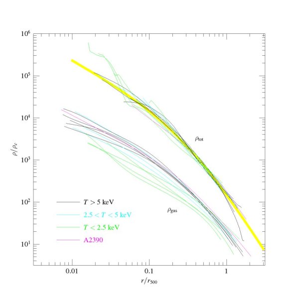
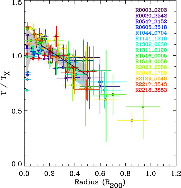
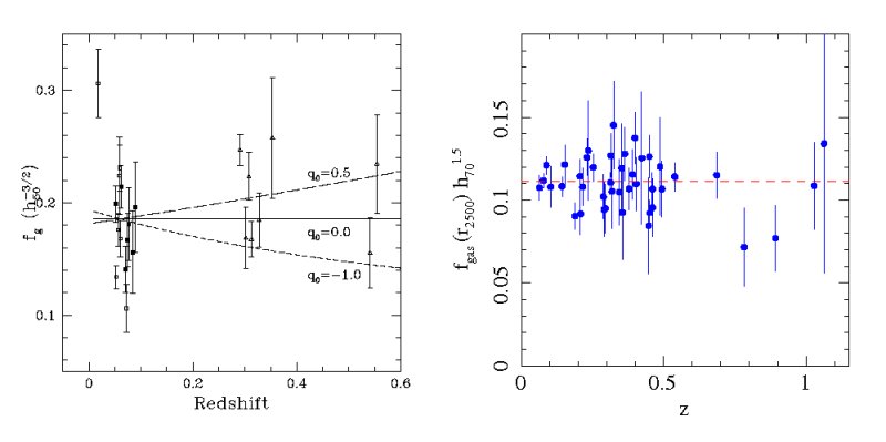
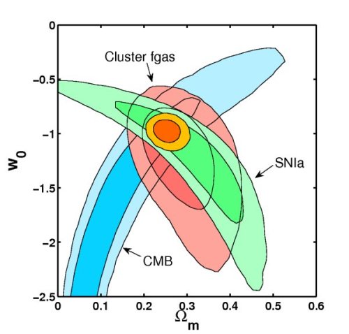
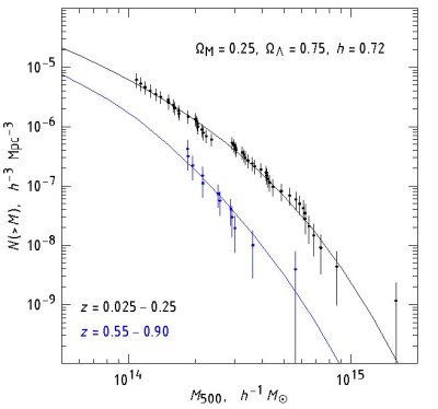
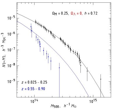
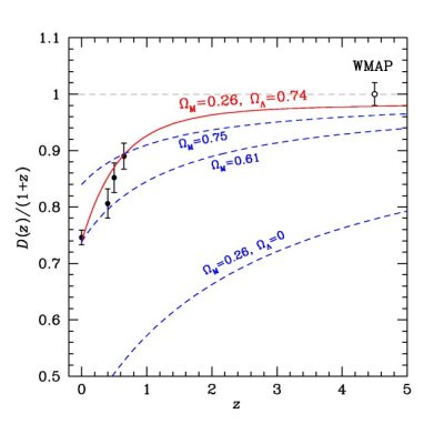
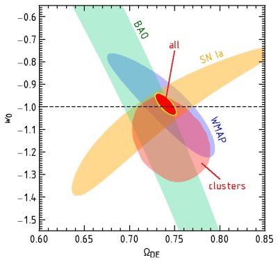
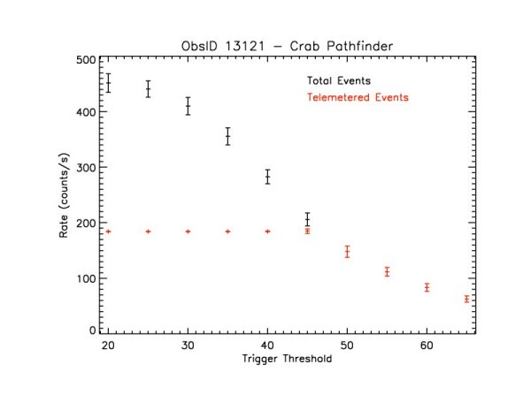
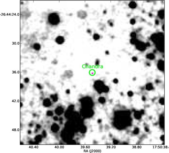
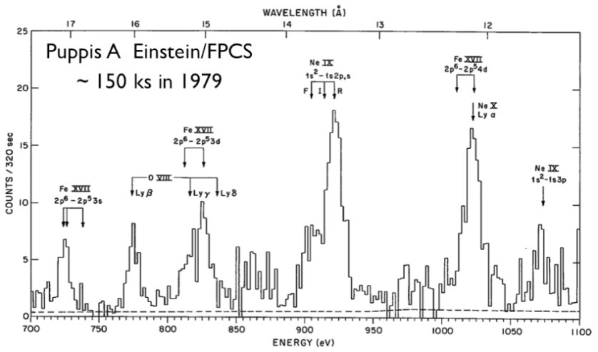
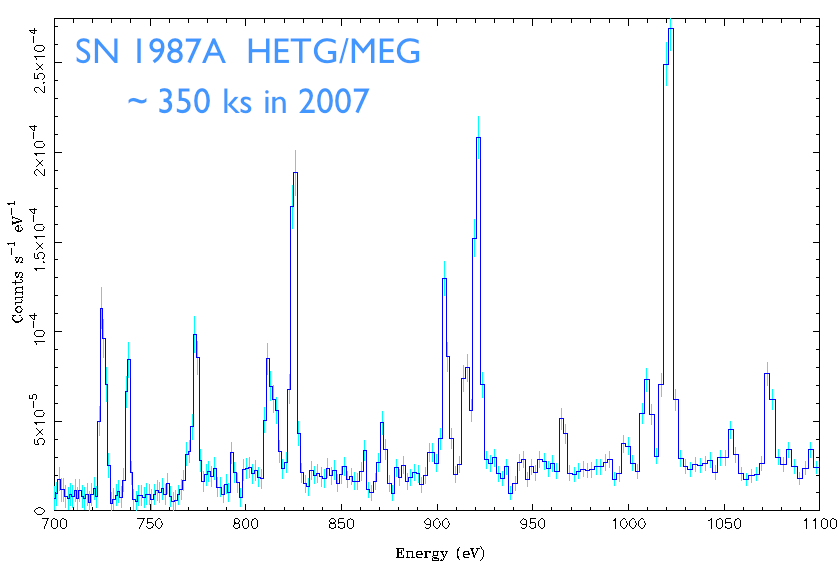
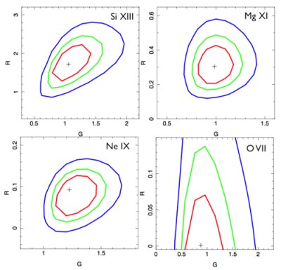
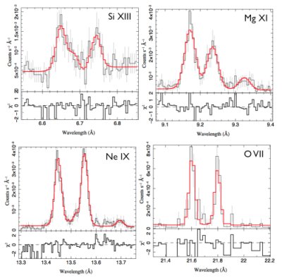
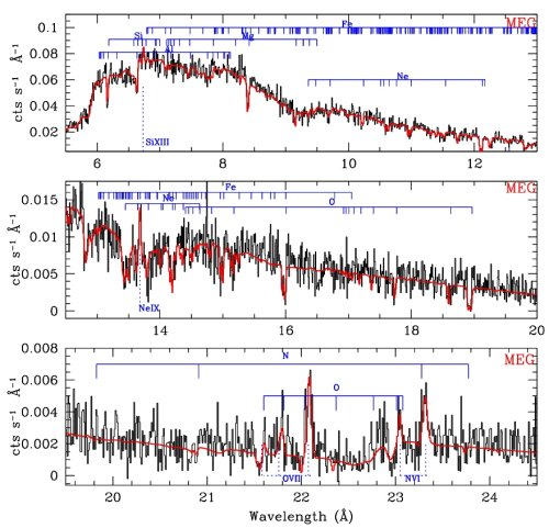
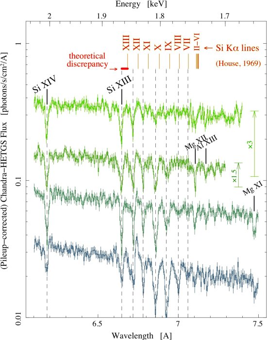
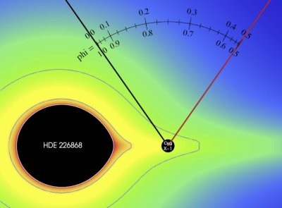
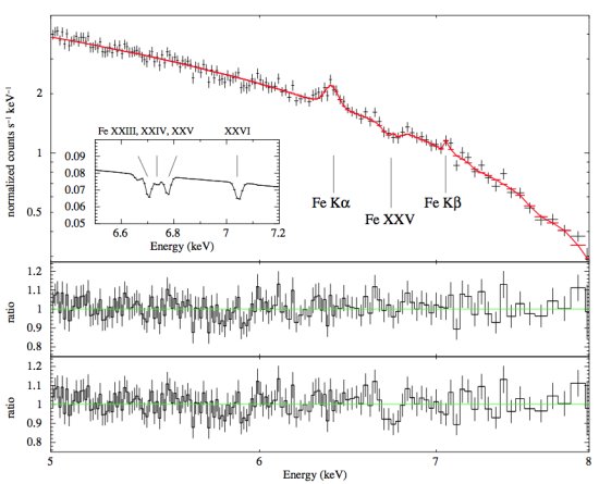
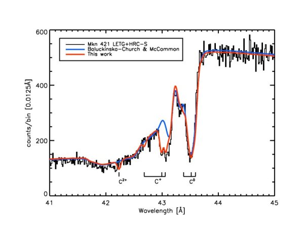
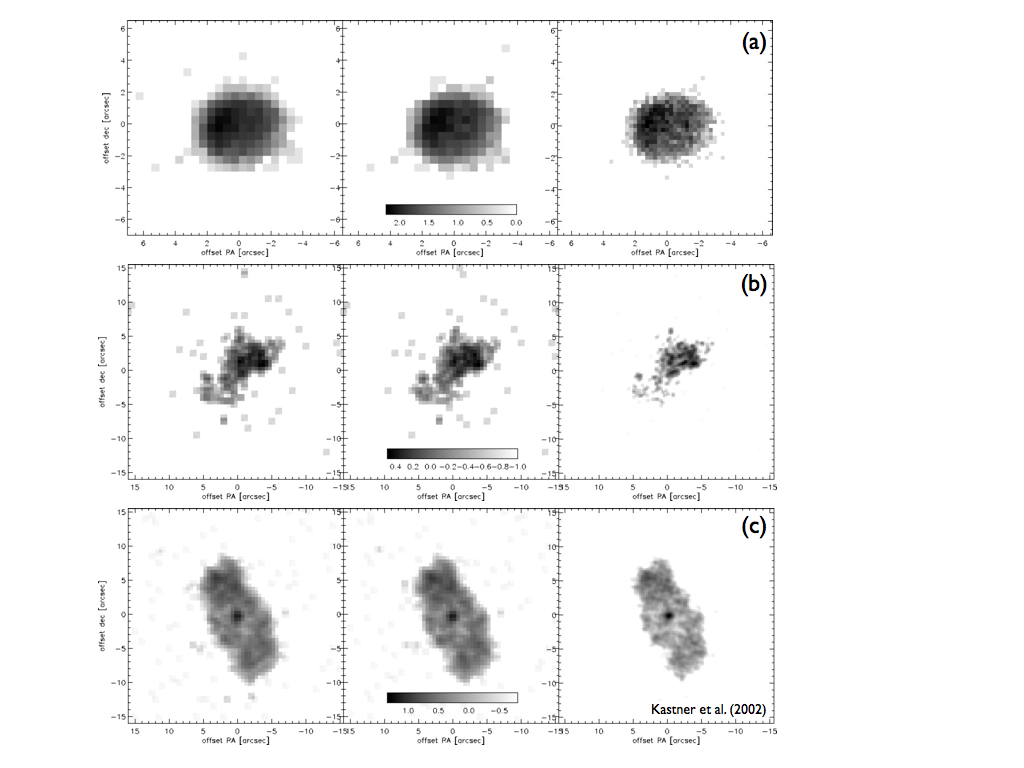
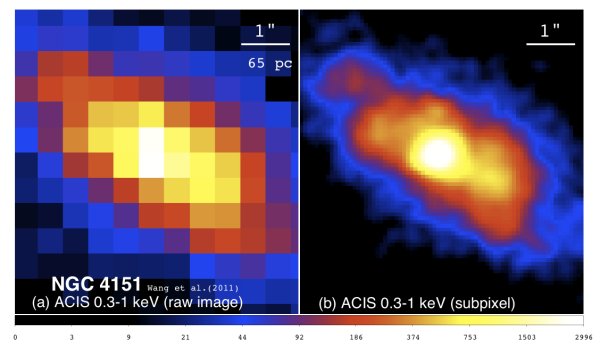
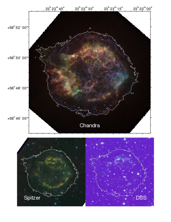
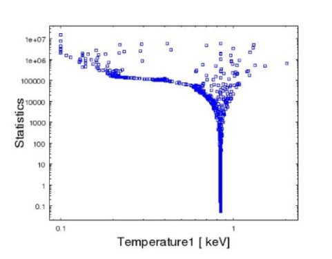
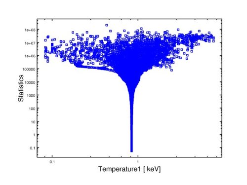
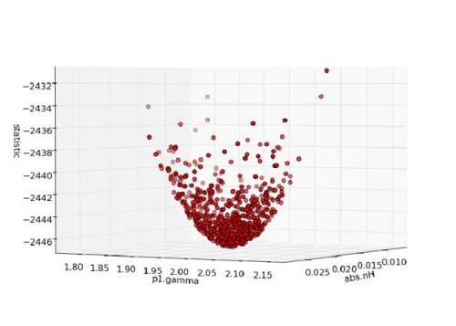
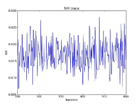
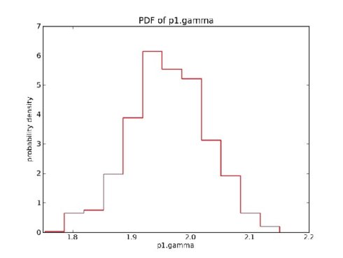
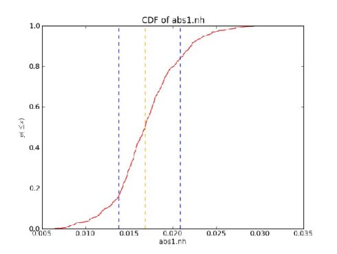
.jpg)