LETG Update
Jeremy J. Drake, for the LETG Team
Trouble in Paradise
Previous Newsletter articles have detailed our continuing efforts to calibrate the HRC-S detector as it ages, let’s say, gracefully. Like my less graceful human case, the aging process undergone by microchannel plate detectors is not understood terribly well. Suffice it to say that space weather can conspire to ruin the bank holiday weekends of spacecraft and scientific instruments alike.
In the case of the HRC-S, the detector gain—essentially the amount of charge liberated by a single X-ray photon event—and the quantum efficiency (QE) are gradually eroded as the potent, shiny, optimistic exuberance of a youthful detector evolves into a wistful, craggy, middle-aged photocathode.
Thank goodness we have painstakingly-devised foolproof calibration to take all of this aging process into account so that observed photon counts of any energy can be reliably converted into fluxes for any epoch in Chandra’s illustrious twenty-year history… How sweet that we can safely bask in the warm, fuzzy comfort this bring… our feet up by the fire after a hard day of calibrating and an impossibly long Chapter 4 of The Chandra X-ray Observatory IOP book to send us to sleep while we sip on a glass of smooth…
It was LETG calibration boffin Pete Ratzlaff who shattered utopia. The data were not behaving.
Paradise Lost QE
In Chandra Newsletter 26, I described the calibration challenges at low energies—below the carbon K edge near 284 eV. At those low energies, we can rely on the constant beacon of the hot white dwarf HZ 43 to guide us. At energies above the carbon edge, there are essentially no bright, constant point sources of X-rays. We are flung into the dark realm of untrustworthy extragalactic sources, forced into Faustian pacts with quasars and blazars to provide our worldly calibration knowledge.
Our primary source in the murky underworld is the bright blazar Markarian 421. Since this, and other, active galactic nuclei are highly variable, these sources cannot be used as standard candles and can only provide relative cross-calibration. We interleave observations using the LETG+HRC-S with LETG+ACIS-S and HETG+ACIS-S, hoping to be able to understand how our calibration needs to adjust in order to be able to draw a nice smooth curve through the observed source flux. One such data set is illustrated in Figure 1. Any such curve is of course not unique, and therein lies the difficulty. Nevertheless, after regular accumulation of data over the years patterns do emerge that appear robust to the vagaries of the subjective judgment of lightcurve beauty.
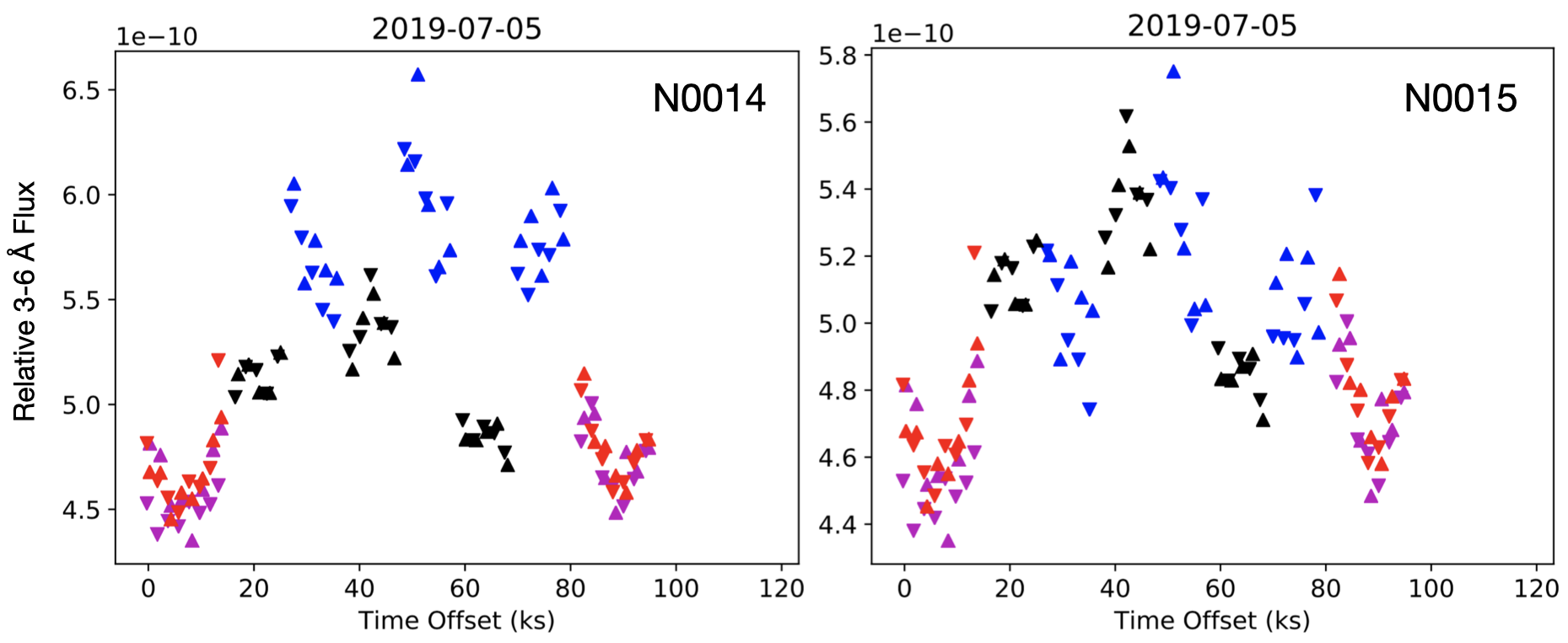
Figure 1: A typical interleaved set of observations of the blazar Mkn 421 obtained in 2019 July used to calibrate the relative instrument throughputs. The figure illustrates the derived flux in the 3–6 Å band as seen by HETG+ACIS-S (red, purple), LETG+ACIS-S (black) and LETG+HRC-S (blue) from old (N0014) and new (N0015) QE calibrations. The light curve should look continuous as the instrument changes if the cross-calibration between instruments is correct.
And all the data have always tended to indicate that the decline in the HRC-S QE was essentially grey—independent of photon energy—until very low energies at locations on the outer plates at wavelengths > 60 Å (200 eV). The QE calibration then presently comprises non-grey corrections derived from routine HZ 43 observations below 200 eV combined with a grey decline at a rate of 2.39% per year to describe the harmonious accord at higher energies.
Then Pete discovered that some of the harmonies were off-key. Not just off-key, but bickering with each other, like a gaggle of belligerent geese. It was the newer data sets that spoiled things. After much thrashing around with the spectra, we realized that the “highest” energies—above 1 keV—did not behave quite the same as the energies below 1 keV. The simple grey scenario was rapidly taking on a technicolor complication.
Figure 1 demonstrates that the precision of each Mkn 421 cross-calibration observation sequence is not that high, especially when we split data into discrete energy or wavelength bands. In order to mitigate the signal-to-noise issue, we resort to the best in astrophysical traditions: average in more data!
The closest known isolated neutron star, RX J1856.5-3754, was observed both near the beginning of the mission, in 2001, and more recently in 2013 and 2019. It is believed constant, other than a bit of pulsating through rotation at a level of about 1%, but is a little too faint to be a useful routine calibration target for the HRC-S QE. It does have measurable flux shortward of 60 Å down to 20 Å though, usefully extending the range of HZ 43 absolute calibrations. Of course, we still do not have a reliable theoretical model for the spectrum of isolated neutron stars like RX J1856.5-3754, and so it can serve as a relative calibrator only.
Careful analysis of the 2001, 2013 and 2019 data supports the grey secular QE correction we apply to the HRC-S. This clearly points the finger at higher energies as the source of our problems. And indeed, slicing the Mkn 421 data into energy ranges revealed a trend of increasing discrepancy with our grey correction toward higher energies. The good news is that the higher energy QE of the HRC-S is declining much more slowly than the low energies.
The new calibration shortward of 60 Å has an increasing secular QE decline from 0.34% per year at the highest energies and shortest wavelengths, increasing with wavelength to reach 2.39% per year at 20 A. The efficacy of this smaller QE decline in the 3–6 Å band can be seen in the right panel of Figure 1 as compared with the left. The latter shows a significant over-correction of the HRC-S QE leading to too high fluxes from the LETG+HRC-S compared with the other instrument combinations.
That we appear to have got it right is demonstrated by HRC-S data obtained for the plerionic supernova remnant G21.5-0.9 illustrated in Figure 2. While we get no spectral information from the HRC, G21.5-0.9 is heavily absorbed by the interstellar medium such that essentially all the X-ray signal is at energies of 1 keV and above. It, therefore, presents a useful probe of the higher energy response of the detector. Although of limited signal-to-noise ratio, recent observations hinted at a rise in flux in recent times by perhaps 7–8%. The source is likely variable at the level of a couple of percent or so, like the Crab nebula, but this much larger apparent change variation meshes well with Mkn 421 data indicating our secular QE corrections have overcooked it at energies > 1 keV.
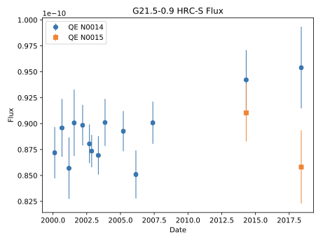
Figure 2: The flux in erg cm-2 s-1 measured for the pulsar wind-driven plerion supernova remnant G21.5-0.9 using the HRC-S with no grating. The blue points correspond to the current calibration, which suggest a rising flux by 7–8% in recent times. The new N0015 calibration (orange points) levels things out to our more physical expectation that the source is more constant than that.
Paradise Regain-mapped
The HRC-S gain is weakly related to photon energy, but is more strongly dependent on detector position: the gain is far from being spatially uniform. Trying to understand and quantify the gain is compounded by its strong time-dependence as it wanes over time. But why do we need to monitor and understand the gain when it is the QE that matters for converting a measured signal to flux?
Unless a photon event signal exceeds a certain threshold it does not get registered and telemetered as a valid event. The problem we are facing now is that the gain is becoming so low in certain detector regions that a small fraction of X-ray events are beginning to slip below the detection threshold—essentially amounting to a loss in QE. At present this is at the 1% or so level within only certain small wavelength ranges, but it is crucial we understand how the gain is evolving so as to allow for and anticipate its effect on the QE. This will also feed into our decision when to raise the detector high tension voltage to increase the gain. I related in Newsletter 26 that we appeared to be at about 7 minutes to midnight on the HRC voltage increase doomsday clock.
Understanding the gain also allows us to filter out some of the background events. The great majority of background events detected by the HRC are due to energetic particles. These tend to have a different, much more broad “pulse height distribution” response—essentially the frequency histogram of detected charge for the combined events—than X-ray photon events. Calibrating these differences allows us to filter out roughly half of the background.
Our crack HRC gain expert, Brad Wargelin, is currently engaged in the epic task of revising the calibration of the time-dependent gain across the detector, an effort that will be related in blank verse in the next Newsletter.
Chandra Burgher in Paradise
The loss of QE at lower, but not higher, energies, points to an effect associated with the primary photon event. Higher energy photons liberate more electrons at the surface of the photocathode. Space weathering appears to have lowered the probability that electrons liberated by a photon event will induce a cascade within the microchannel plates.
So, here we all are. Pete shattered utopia, but he managed to piece it back together again with only the odd crack in the plaster still showing. Now we know the direction it is going in, our current calibration for the higher energies will be scrutinized and revisited as we get more and more data. For now, we can safely bask in the warm, fuzzy comfort the new calibration brings… our feet up by the fire in our house of cards after a hard day of calibrating and an impossibly long Chapter 4 of The Chandra X-ray Observatory IOP book to send us to sleep while we sip on a glass of smooth…
LETG spectra in abundance
One of my favorite little pieces of unsolved physics of the outer atmospheres of stars is the peculiar patterns of chemical abundances they show. The corona of a star contains very little mass compared with the rest of the star, or even with the stellar wind. The Sun loses as much mass through its very tenuous wind in a day or so–a few 1040 protons–as is magnetically confined in the whole of the corona at any given time.
You would expect a plasma sitting on top of a quasi-infinite reservoir of material to mirror the chemical composition of that reservoir. But something plays with that pattern and changes it. A capricious coronal sprite, acting a bit like a Maxwell demon, letting more of certain elements from the photosphere pass through to the corona than others. And stars appear to have different sprites, changing the patterns according to their own whimsical tastes.
The solar corona has more of elements that are easily ionized (Fe, Mg, Si…) than those that are not (C, N, Ne, O…), and the chemical composition tends to follow a step function based on element FIP – first ionization potential. The magnitude of the step varies in different regions of the solar corona. In other stars, especially very magnetically-active stars, the pattern was first seen to be reversed—low FIP elements appeared depleted relative to high FIP elements. My hope was always (the optimism of youth…) that the chemical composition would betray aspects of the fundamental physics driving stellar coronae—much like how the abundance patterns in evolved stellar photospheres betray the nucleosynthesis and mixing at work in stellar interiors. The key is to build up an accurate picture of how coronal abundances map out over stellar parameter space—how they depend on stellar mass, or spectral type, and magnetic activity level.
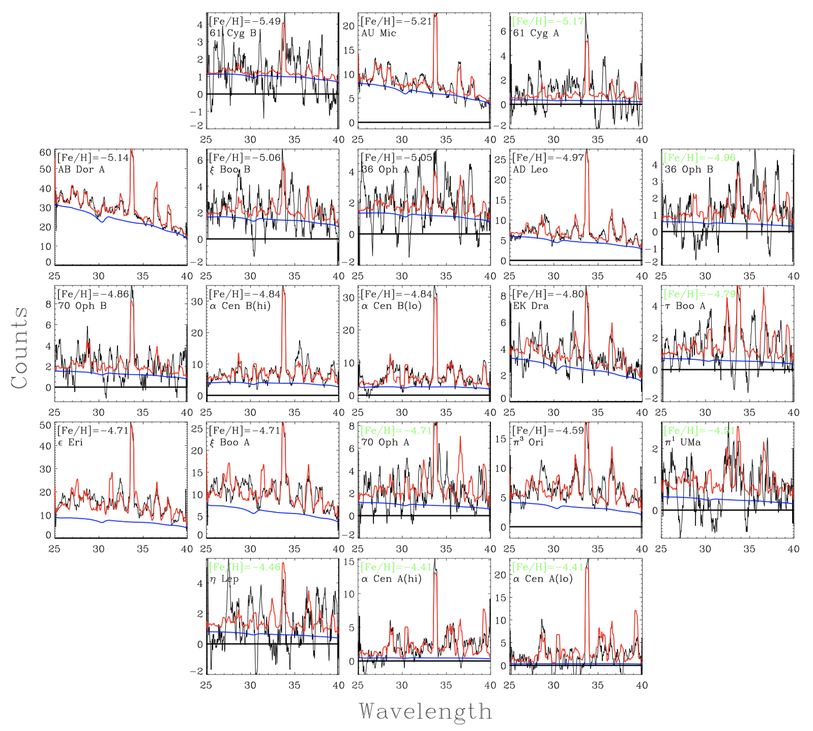
Figure 3: The 25–40 Å range in the stars of the LETG+HRC-S coronal abundance survey of Wood et al (2018) used to determine the continuum level and estimate absolute coronal abundances. The thinner black lines show the smoothed observed spectra, the blue curves represent the inferred continuum level, and the red lines show the derived synthetic spectra. The estimated iron abundance is indicated in each panel in black, with values in green indicating assumed values in cases lacking a significant continuum detection.
An abundance of Ca, U, Ti, O, N (well, ok, not U)
An important step in this direction has been made by Brian Wood of the Naval Research Laboratory, and collaborators, with an extensive LETG survey of late-type stars that provides a good deal of the mapping required to begin to understand the underlying physics (Wood et al 2018).
Figure 3 presents a creative 21-panel layout showing the 25–40 Å spectral region in which some key lines and the continuum level have been observed in the survey stars using the LETG+HRC-S. Wood and co-workers performed a differential emission measure analysis to obtain element abundances – working out the emitting power of the plasma as a function of temperature, and adjusting abundances to match the observed line fluxes and line-to-continuum ratio. The result is a picture of the “FIP bias” over a range of spectral types. Wood et al define the FIP bias as the average abundance of the high FIP elements (C, N, O and Ne) relative to Fe, the best-measured low-FIP element. This is plotted for the stars of the survey in Figure 4, together with a linear fit to the data.
The FIP bias at the effective temperature of the Sun shows the well-known solar-like FIP effect, with an enhancement of Fe and other low-FIP elements. However, going to cooler spectral types this transitions gradually into an inverse FIP effect, passing through a FIP bias of zero in mid-K spectral types and demonstrating that the FIP effect is a strong function of spectral type.
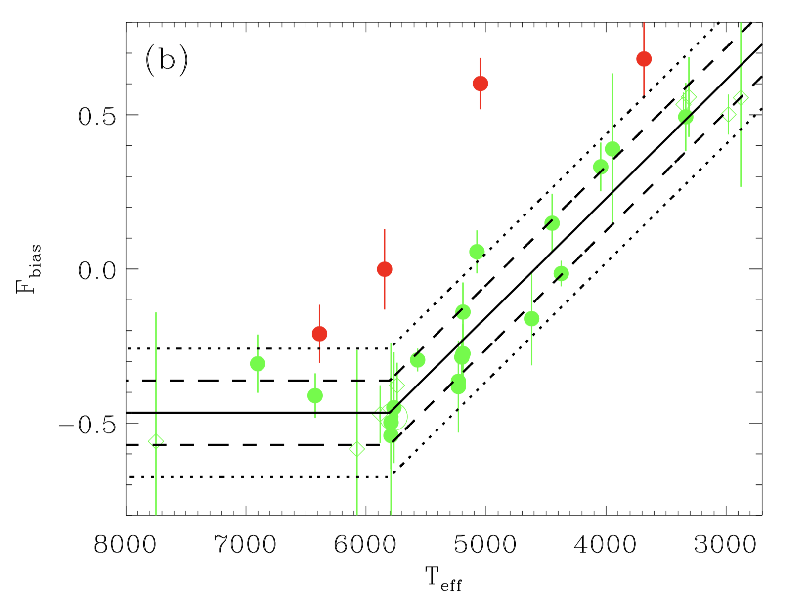
Figure 4: The “FIP bias”, Fbias vs. stellar effective temperature, Teff, together with linear fits and their 1σ (dashed lines) and 2σ (dotted lines) bounds. to the data. The red points correspond to very active stars that lie significantly above the main trend.
But Figure 4 also shows four stars that do not appear to fit into the relation, and indicate a greater shifter to inverse FIP than the other stars. These four stars are magnetically active, including, for example, the zero-age main-sequence star AB Doradus, with a rotation period of only half a day. This inverse FIP pattern showed up in early coronal abundance work because observations with satellites such as ASCA, BeppoSAX and EUVE first concentrated on the brightest sources, which of course are the most active. So, magnetic activity complicates the simple spectral-type dependence.
So what is going on? Several different models for the FIP effect have been developed over the years. However, the most promising is the finding by Martin Laming, also of the Naval Research Laboratory, that the ponderomotive force on ions subject to Alfvén waves passing through, or reflecting at, the chromosphere can provide the ion-neutral separation (eg, Laming 2012). The Alfvén waves can be generated by surface and subsurface convection, and also by magnetic turbulence and reconnection in the corona, with the direction of motion giving rise to low-FIP enhancement or suppression—hence the dependence of the FIP bias on both stellar effective temperature, on which convection properties depend, and on magnetic activity level that feeds the dynamics of the corona.
Alfvén waves are a prime suspect in the currently unsolved 80 year old problem of the heating of the solar corona, and are likely the main driver of the solar wind. The great appeal of the ponderomotive force model, then, is that abundances would give us new insights into Alfvén waves and their generation in stellar coronae… Surely only a step or two away from understanding that old coronal heating problem itself.
JJD thanks the LETG team for useful comments, information, and discussion.
References
- Laming, J. M. 2012, ApJ, 744, 115
- Wood, B. E., Laming, J. M., Warren, H. P., and Poppenhaeger, K., 2018, ApJ, 862, 66