The Chandra Source Catalog 2.0 Science Threads: A New Approach to Accessing the Catalog via Jupyter Notebooks
Rafael Martinez-Galarza on behalf of the CSC team
Introduction
Version 2.0 of the Chandra Source Catalog (CSC 2.0) offers an unprecedented opportunity for discovery. It provides astrometric, photometric, spectroscopic, and variability properties for over 317,000 X-ray sources in the sky, which were calibrated and computed in a uniform fashion. The majority of the CSC 2.0 sources are serendipitous and have never been investigated in detail. Perhaps less known to users, the catalog also provides science-ready data products for each field, (and, when applicable, for each source/detection) that facilitates the characterization of those sources. These data products include event lists, detection lists, sensitivity and background maps, spectra, light curves, and MCMC-computed probability density functions for the estimated astrometric and photometric quantities, which amount to about 35TB of data (uncompressed). With CSC 2.0 we have also developed several interfaces to access the tabulated properties and data products. Here we present a new series of science threads that show how to interact with the catalog from a Jupyter notebook session by making use of Virtual Observatory (VO) interfaces, such as Simple Cone Search (SCS) and Table Access Protocol (TAP). We demonstrate typical science workflows, such as, downloading of specific data products, cross-matching with multi-wavelength catalogs, performing spectral fitting, identifying short-term and long term variability, and estimating the cumulative sky coverage.
Accessing and processing data from a Jupyter notebook
The science threads presented here are accessible from our documentation pages. PyVO version 1.1 allows users to query Virtual Observatory services from Python. Our threads show how you can use it to query CSC 2.0 using the VO interfaces for tabulated properties. They also show how to use CIAO tools to retrieve catalog data products. The science threads assume that you have installed CIAO 4.13 using conda. Here we use astropy 4.0.1, matplotlib 3.3.1, and numpy 1.19.1.
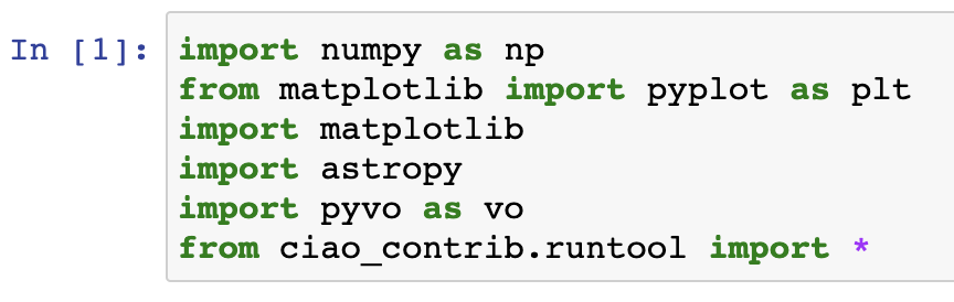
The basic imports are shown below.
As an example, a cone search for sources within 1 degree of M33 can be performed with:
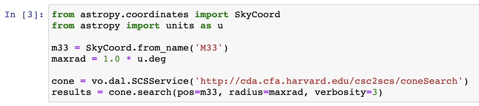
The results variable will contain a table with the CSC 2.0 properties for the sources found within the defined area. The keyword verbosity controls how many catalog columns you get, ‘3’ returns all of the columns.
In the next subsections we show extracts of 3 different workflows: 1) inspecting the short- and long-term variability of sources in a particular region of the sky, 2) accessing and plotting data products such as light curves and data products, 3) cross-matching CSC with an infrared catalog, 4) getting the cumulative sky sensitivity coverage for a region of interest in the sky. We only provide the most representative plots in each case, but the full workflows can be accessed through the downloadable notebook in our documentation pages.
Inspecting hardness ratios and variabilities
CSC 2.0 provides measures of fluxes in several energy bands ranging from 0.5 keV to about 7 keV, and estimates of variability in each of these bands, as well as in the full broad (ACIS) and wide (HRC) bands. Variability is estimated both in short (duration of a single Chandra observation) and long (typical duration between Chandra observations of the same source) timescales. Suppose you are interested in visualizing the hardness ratios for the sources we have selected above, and see how the hardness ratios relate to variability. For example, you might be interested in selecting X-ray binaries that have a hard spectrum and that show long term-variability (i.e. their flux significantly changes from observation to observation). Figure 1 shows the relationship between the hard-to-medium and hard-to-soft hardness ratios and the variability in short timescales (typically a duration within a single Chandra observation, i.e., a few hours) and in long timescales (typically a duration between observations, i.e., months to years).
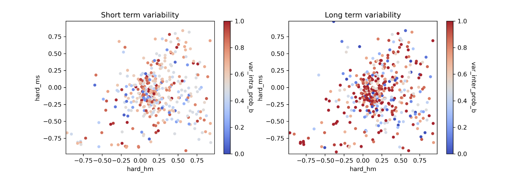
Figure 1: The hard (2 keV-7 keV) to medium (1.2 keV-2 keV) vs hard to soft (0.5 keV-1.2 keV) hardness ratios for CSC 2.0 sources within 1 degree of M33. In the left panel they are color-coded by their probability of short-term (intra-observation) variability, whereas in the right panel the color code reflects long-term (inter-observation) variability.
Accessing data products
Suppose you are interested in looking at the spectrum and the light curve of a source of interest (e.g. 2CXO J002404.2-720457, whose coordinates are RA = 6.01784 deg, DEC = -72.08276 deg), which is a transient source in globular cluster 47 Tuc. You can do this from within your Jupyter session using CIAO tool search_csc, which takes the coordinates as input:
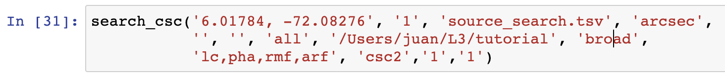
Note that we have requested file types for the light curve (lc) and the spectral files (pha, rmf, arf) for the broad band. This will download all of the associated files for this source. We can then visualize them, and also perform scientific operations, such as fitting the spectrum, all from within the same notebook session. In Figure 2, we show examples of the downloaded data products.
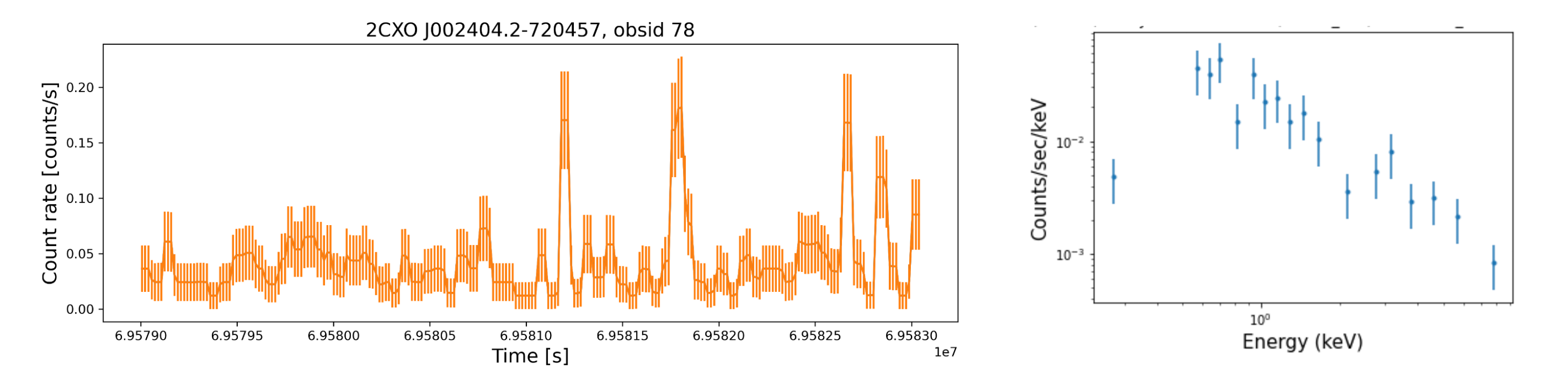
Figure 2: The light curve (left panel) and spectrum (right panel) of CSC 2.0 source 2CXO J002404.2-720457. These are science-ready data products downloaded from within the Jupyter notebook session.
Cross-matching with other (optical/IR) catalogs
X-ray properties are often an excellent complement to optical and IR observations of specific sources (and vice versa). It is possible to cross-match CSC 2.0 sources with other catalogs. For example, Figure 3 shows a selection of about 500 sources in the Orion nebula. They represent color hardness and X-ray flux-IR magnitude diagrams for young stars constructed from cross-matching CSC 2.0 with the 2MASS catalog.
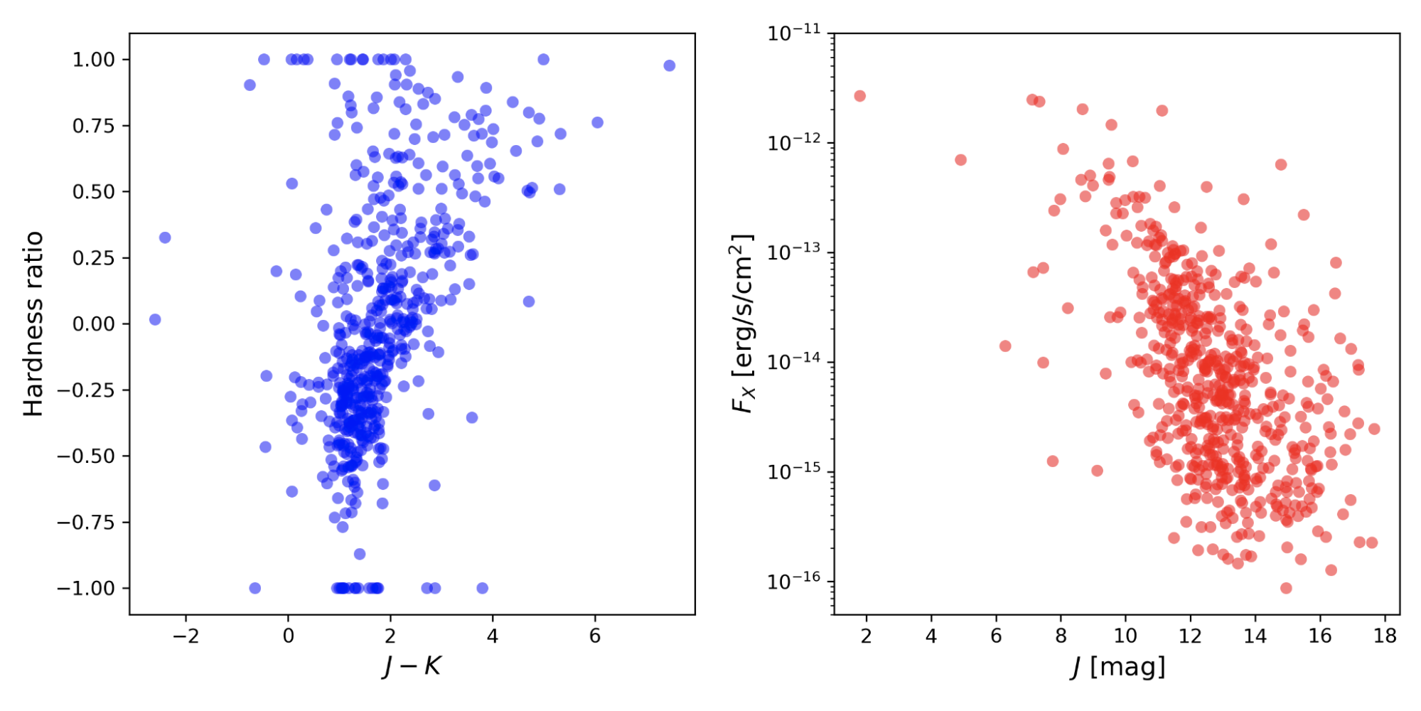
Figure 3: Left panel – Color hardness diagram for a selection of young stellar objects in M42. Right panel – near infrared magnitude plotted against X-ray flux for the same sources.
Cumulative sky coverage
Number counts or luminosity functions of different classes of X-ray sources allow the determination of those sources’ contributions in various astrophysical problems. To determine the number counts of sources in flux-limited surveys, one needs to know the cumulative sky coverage Ω(F>Fmin), i.e., the survey area in which a source brighter than flux Fmin could be detected, as a function of Fmin (see, e.g. Miyaji et al., 2015). In a similar way as we did for the light curves and spectra, in a Jupyter notebook session we can download sensitivity maps for each of the catalog stacks (collections of co-added observations) that intercept a region of interest in the sky. We can then reproject and combine these maps into a mosaic to create the combined sensitivity map for the region of interest. In Figure 4, we show the resulting mosaic for a 12 arcmin region near the Lockman Hole, as well as the resulting cumulative histogram of sky coverage.
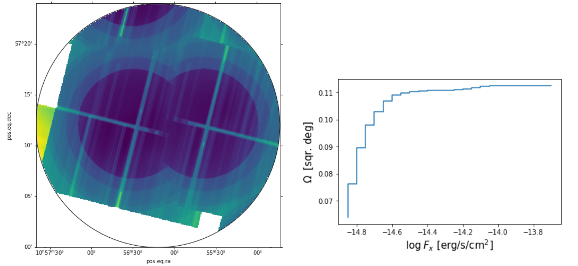
Figure 4: Left panel – a composite mosaic of reprojected CSC 2.0 sensitivity maps in a region within the Lockman Hole. Right panel – the cumulative histogram of sky coverage for the same region.
Conclusion
Tabulated properties and data products from CSC 2.0 can be readily accessed from a Python session, and easily combined with astropy, Sherpa, and other analysis tools in order to perform many scientific tasks in a single session. The CSC 2.0 documentation pages will be regularly updated with new Jupyter notebooks showing examples of different science applications. If you have ideas for specific science threads, please contact: cxchelp@cfa.harvard.edu.