Gallery: Regions
Examples
- Single contour
- Multiple contours
- Magic Wand Tool: dmimglasso
- Convex Hull
- Flux Fraction Ellipse Finding
- Rectangles instead of Ellipses
1) Single contour
CIAO has several other tools to create regions automatically from the input image beyond those shown in the detect tools gallery.
One common task is to draw contours. This can be done with the dmcontour tool.

dmimgadapt a1664.img a1664.asm cone 1 20 40  linear 100 clob+
dmcontour a1664.asm 0.75 a1664_0.75_cntr.reg clob+
The following commands can be used to visualize the output
ds9 a1664.asm -scale log -region a1664_0.75_cntr.reg -cmap load $ASCDS_CONTRIB/data/heart.lut
The image input to dmcontour should be smoothed to avoid getting thousands of small regions around individual single-count pixels. dmimgadapt is use here to smooth the image of Abell 1664 using a variable size cone; requiring at least 100 counts under the smoothing kernel.
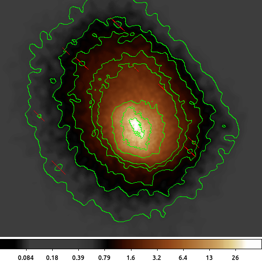
dmcontour is then used to create regions. A single contour is created at level=0.75 counts.
As this example shows, there are several small regions that are excluded from within the main contour; as well as several other smaller contour regions outside the primary emission. The dmcontour output is a FITS region composed of polygons; the regions are constructed such that the pixel values greater than the contour level are included in the polygon.
2) Multiple contours
We can also generate multiple contour regions with dmcontour similar to the previous example,
dmcontour a1664.asm "0.5,0.75,1.0,1.5,2.0,5,12,25" a1664_stk_cntr.reg clob+
The following commands can be used to visualize the output
ds9 a1664.asm -scale log -region a1664_stk_cntr.reg -cmap load $ASCDS_CONTRIB/data/heart.lut
Individual contour levels can be extracted
or in a single step:
dmstat "a1664.asm[sky=region(a1664_stk_cntr.reg[contour_level=2.0])]" sig- med- cen-
Remember, each contour is one or more polygons that includes all pixel values greater than the contour level. If you want the pixel values between two contour levels, then you would need to filter twice: once to include the lower level, and then a second time to exclude the upper level.
3) Magic Wand Tool: dmimglasso
The dmcontour command computes the contour polygons for all pixels in the input image. As we saw in first example, it generates polygons around disjoint groups of pixels. The dmimglasso tool can be used to create a similar contour-level polygon which restricts the output to those pixels which have an unbroken path to the input x,y location.
The tool gets its name from the lasso (or magic wand) selection tool available in various photo editing packages.

dmimglasso a1664.asm a1664.lasso 4126 4008 0.75 INDEF coord=physical clob+ max=100000
The following commands can be used to visualize the output
ds9 a1664.asm -scale log -region a1664.lasso -cmap load $ASCDS_CONTRIB/data/heart.lut
In this example dmimglasso starts at x=4126, y=4008 and collects all the pixels that are greater than 0.75. The output region is shown. Compared to the dmcontour example, we see that the two separate, disjoint regions are not identified.
A closer inspection of the region will show a "city-block" style contour where each line segment is a right angle and fully encloses the pixel. The dmcontour output is a polygon with arbitrary angle and location within a pixel.
The max=100000 value is set to ensure that the program can recursively compute the needed contour. This is a hidden parameter used to prevent the tool from going into an infinite loop and consuming too much memory.
4) Convex Hull
Both the dmcontour and dmimglasso polygon outputs have a large number of sides. Each pixel along the contour level edge adds at least one line segment (sometimes two or three). This produces a highly accurate contour, but when used as a filter it may result in long CPU runtimes.
The dmimghull tool computes a simple convex hull (polygon) around the above-threshold pixels in the image.
dmimghull a1664.asm a1664_0.75.hull tol=0.75 clob+
The following commands can be used to visualize the output
ds9 a1664.asm -scale log -region a1664_0.75.hull -cmap load $ASCDS_CONTRIB/data/heart.lut
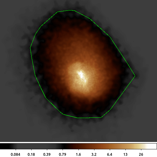
The convex hull shown here bumps out to the west-south-west to include the isolated emission which can also be seen in the above example. It also does not have the interior excluded region shown in the earlier examples. But this polygon only has 34 sides compared to the 1,697 sided polygon created by dmimglasso.
5) Flux Fraction Ellipse Finding
Another way to automatically generate regions is to create a region that encloses a certain fraction of the total flux (or in this case counts). The dmellipse tool does this in a somewhat brute force method by guessing the parameters for an ellipse and then increasing or decreasing the size until it finds an ellipse that meets the desired flux fraction.
It turns out that this is in general a poorly constrained problem, as there are an infinite number of ellipses that can satisfy a simple flux-limit constraint. dmellipse imposes additional limits that the centroid of the data inside the ellipse is the center of the ellipse and that the radii are consistent with the moments.
dmellipse a1664.asm a1664.ellipses "lgrid(0.1:0.96:0.05)" step=100 clob+
The following commands can be used to visualize the output
ds9 a1664.asm -scale log -region a1664.ellipses -cmap load $ASCDS_CONTRIB/data/heart.lut
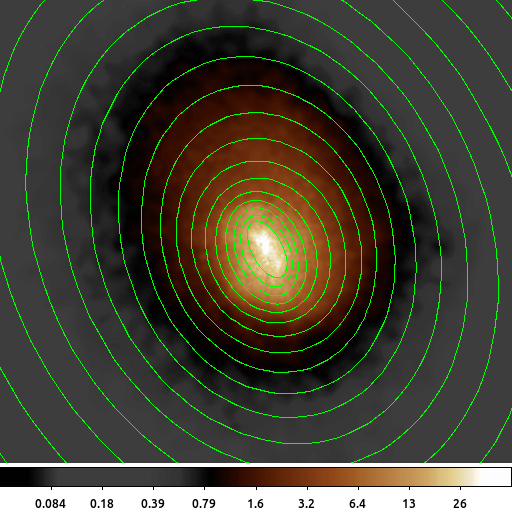
Here we show the dmellipse output for a stack of requested fractions. The stack is expressed using the lgrid (linear grid) syntax where we requested fractions going from 0.1 (10%) to 0.96 (96%) in 5% increments. We selected 96 rather than 95 so that the 95% limit would be included.
The initial step size is increased because we are making large ellipses. This make the tool run much faster. If working with smaller images (eg of the PSF) then a smaller initial step size can be used.
In this example the 10% ellipse is the inner most ellipse. The 15% ellipse fully encloses the 10% ellipse, and so on; however, the center is computed separately for each ellipse based on the centroid of the data enclosed by that ellipse. The center of the ellipses drifts slightly as the fraction of flux increases. This is a good indicator that the observed flux is not symmetric about a single point.
Note: The gaps in the largest ellipses are an artifact of how ds9 draws them. The actual results are fully enclosed ellipses.
6) Rectangles instead of Ellipses
dmellipse has the option to use rotated boxes instead of ellipses. While this may not be scientifically useful for this particular dataset, it does make it easier to see how the algorithm works.

dmellipse a1664.asm a1664.rotboxes "lgrid(0.1:0.96:0.05)" shape=rotbox step=100 clob+
The following commands can be used to visualize the output
ds9 a1664.asm -scale log -region a1664.rotboxes -cmap load $ASCDS_CONTRIB/data/heart.lut
This example uses the same parameters as before but now we require a rotated box to enclose 10%, 15%, 20%, ... 95% of the counts.
The subtle difference in the rotation angle at each flux level is much easier to see now.
dmellipse does have parameters to control the initial ellipse or rotbox parameters and also allows the parameters to be frozen.